Active Filters

Passive RLC filters are simple and easy to design and use. However, can we implement them on-chip? Let us look at a simple example to give us a bit more insight regarding this question.

Example: A passive band-pass filter

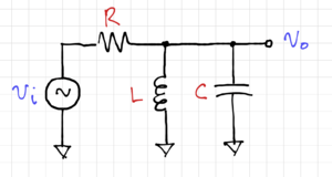
Figure 1: A passive LC band-pass filter.

Consider the LC band-pass filter shown in Fig. 1. We can write the transfer function as:

${\begin{aligned}H\left(s\right)&={\frac {v_{o}}{v_{i}}}={\frac {sL\|{\frac {1}{sC}}}{R+sL\|{\frac {1}{sC}}}}={\frac {sL\cdot {\frac {1}{sC}}}{R\cdot \left(sL+{\frac {1}{sC}}\right)+sL\cdot {\frac {1}{sC}}}}\\&={\frac {sL}{s^{2}RLC+R+sL}}={\frac {s\cdot {\frac {1}{RC}}}{s^{2}+s\cdot {\frac {1}{RC}}+{\frac {1}{LC}}}}\\\end{aligned}}$

(1)

If we let $Q=\omega _{0}RC={\tfrac {R}{\omega _{0}L}}$ and $\omega _{0}={\tfrac {1}{\sqrt {LC}}}$, then we can rewrite our expression for $H\left(s\right)$ as:

$H\left(s\right)={\frac {s\cdot {\frac {\omega _{0}}{Q}}}{s^{2}+s\cdot {\frac {\omega _{0}}{Q}}+\omega _{0}^{2}}}$

(2)

Notice that the transfer function has two zeros, $s_{z}=\left(0,\infty \right)$, and two poles located at:

$s_{p}=-{\frac {\omega _{0}}{2Q}}\pm {\frac {1}{2}}\cdot {\sqrt {{\frac {\omega _{0}^{2}}{Q^{2}}}-4\omega _{0}^{2}}}$

(3)

We get complex conjugate poles if $4\omega _{0}^{2}>{\tfrac {\omega _{0}^{2}}{Q^{2}}}$ or when $Q^{2}>{\tfrac {1}{4}}$, or equivalently, when $Q>{\tfrac {1}{2}}$. If the band-pass filter has $\omega _{0}=2\pi \cdot \left(1\,\mathrm {kHz} \right)$, $Q=20$, and $R=50\,\mathrm {\Omega }$:

$L={\frac {R}{\omega _{0}Q}}={\frac {50\,\mathrm {\Omega } }{2\pi \cdot \left(1\,\mathrm {kHz} \right)\cdot 20}}=398\,\mathrm {\mu H}$

(4)

$C={\frac {Q}{\omega _{0}R}}={\frac {20}{2\pi \cdot \left(1\,\mathrm {kHz} \right)\cdot \left(50\,\mathrm {\Omega } \right)}}=64\,\mathrm {\mu F}$

(5)

Figure 2: A lossy inductor.

Let us now consider a lossy inductor with $Q_{\text{ind}}=40={\tfrac {\omega _{0}L}{R_{s}}}$. The loss can then be modeled by the series resistance, $R_{s}$, as shown in Fig. 2, with:

$R_{s}={\frac {\omega _{0}L}{Q_{\text{ind}}}}={\frac {2\pi \cdot \left(1\,\mathrm {kHz} \right)\cdot \left(398\,\mathrm {\mu H} \right)}{40}}=0.0625\,\mathrm {\Omega }$

(6)

We can convert the series RL circuit to its parallel circuit equivalent in Fig. 2 at $\omega =\omega _{0}$ by first writing out the admittance of the series RL circuit as:

${\begin{aligned}Y&={\frac {1}{R_{s}+j\omega _{0}L}}={\frac {1}{R_{s}+j\omega _{0}L}}\cdot {\frac {R_{s}-j\omega _{0}L}{R_{s}-j\omega _{0}L}}\\&={\frac {R_{s}-j\omega L}{R_{s}^{2}+\omega _{0}^{2}L^{2}}}={\frac {R_{s}}{R_{s}^{2}+\omega _{0}^{2}L^{2}}}-{\frac {j\omega L}{R_{s}^{2}+\omega _{0}^{2}L^{2}}}\\&={\frac {1}{R_{s}}}\cdot {\frac {1}{1+{\frac {\omega _{0}^{2}L^{2}}{R_{s}^{2}}}}}+{\frac {1}{j\omega _{0}L}}\cdot {\frac {1}{1+{\frac {R_{s}^{2}}{\omega _{0}^{2}L^{2}}}}}\\&={\frac {1}{R_{s}}}\cdot {\frac {1}{1+Q_{\text{ind}}^{2}}}+{\frac {1}{j\omega _{0}L}}\cdot {\frac {1}{1+{\frac {1}{Q_{\text{ind}}^{2}}}}}\\&={\frac {1}{R_{p}}}+{\frac {1}{j\omega _{0}L^{\prime }}}\end{aligned}}$

(7)

Thus, we get:

$R_{p}=R_{s}\cdot \left(1+Q_{\text{ind}}^{2}\right)$

(8)

$L^{\prime }=L\cdot \left(1+{\frac {1}{Q_{\text{ind}}^{2}}}\right)$

(9)

For $Q_{\text{ind}}=40$, we get almost no change in the inductor value, or equivalently $L^{\prime }\approx L$. We can then redraw our band-pass filter with the lossy inductor model, as shown in Fig. 4. Thus, the new transfer function is then:

${\begin{aligned}H\left(s\right)&={\frac {v_{o}}{v_{i}}}={\frac {s\cdot {\frac {1}{RC}}}{s^{2}+s\cdot {\frac {1}{C}}\cdot \left({\frac {1}{R_{p}}}+{\frac {1}{R}}\right)+{\frac {1}{LC}}}}\\&={\frac {s\cdot {\frac {\omega _{0}}{Q^{\prime }}}}{s^{2}+s\cdot {\frac {\omega _{0}}{Q^{\prime }}}+\omega _{0}^{2}}}\end{aligned}}$

(10)

Note that $\omega _{0}$ remains approximately the same, and the overall quality factor, $Q^{\prime }$, becomes:

${\begin{aligned}{\frac {\omega _{0}}{Q^{\prime }}}&={\frac {1}{C}}\cdot \left({\frac {1}{R}}+{\frac {1}{R_{p}}}\right)={\frac {1}{RC}}+{\frac {1}{R_{p}C}}\\{\frac {1}{Q^{\prime }}}&={\frac {1}{\omega _{0}RC}}+{\frac {1}{\omega _{0}R_{p}C}}={\frac {1}{Q}}+{\frac {1}{\omega _{0}R_{p}C}}\\&={\frac {1}{Q}}+{\frac {1}{\omega _{0}R_{s}\left(1+Q_{\text{ind}}^{2}\right)C}}\\&={\frac {1}{Q}}+{\frac {Q_{\text{ind}}}{1+Q_{\text{ind}}^{2}}}\\&\approx {\frac {1}{Q}}+{\frac {1}{Q_{\text{ind}}}}\end{aligned}}$

(11)

We can then plot the magnitude response of both the ideal LC band-pass filter and the filter with a lossy inductor, as shown in Fig. 5. Note the significant degradation of the magnitude response peak, and the increase in bandwidth when we used an inductor with finite quality factor.

For the ideal case, with a lossless inductor:

$Q_{\text{filter}}={\frac {f_{0}}{\Delta f}}={\frac {1\,\mathrm {kHz} }{50\,\mathrm {Hz} }}=20$

(12)

For the filter with a lossy inductor, with $Q_{\text{ind}}=40$, and from the magnitude response in Fig. 5, we can get:

$Q_{\text{filter}}^{\prime }={\frac {f_{0}}{\Delta f}}={\frac {1\,\mathrm {kHz} }{76\,\mathrm {Hz} }}=13.16$

(13)

Note that our approximation gives a reasonable estimate of the filter quality factor:

$Q_{\text{filter}}^{\prime }\approx \left({\frac {1}{Q}}+{\frac {1}{Q_{\text{ind}}}}\right)^{-1}=\left({\frac {1}{20}}+{\frac {1}{40}}\right)^{-1}=13.33$

(14)