Difference between revisions of "Probability review for warm up"
Ryan Antonio (talk | contribs) |
Ryan Antonio (talk | contribs) |
||
| Line 84: | Line 84: | ||
<math> \{2,3,4,5,6,7,8,9,10,11,12\} </math> | <math> \{2,3,4,5,6,7,8,9,10,11,12\} </math> | ||
| − | Now, each outcome would have | + | Now, each outcome would have some probability associated with it. The list below shows the pair-wise mapping. We'll leave it as an exercise for you to determine how to get these probabilities. |
| + | |||
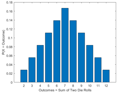
| + | [[File:Bar graph.PNG|thumb|400px|right|Bar graph for the probability distribution of the sum of two die rolls.]] | ||
* <math> P(X = 2) = \frac{1}{36} </math> | * <math> P(X = 2) = \frac{1}{36} </math> | ||
| Line 98: | Line 100: | ||
* <math> P(X = 12) = \frac{1}{36} </math> | * <math> P(X = 12) = \frac{1}{36} </math> | ||
| − | + | The mapping between the outcomes and their corresponding probabilities is called a ''probability distribution''. It describes the chances of the random variable to be one of the outcomes. It is common to visualize discrete random variables with bar graphs. Figure 3 shows the probability distribution of our two die rolls example. | |
== Exercises == | == Exercises == | ||
Revision as of 09:12, 5 February 2022
Contents
Probability Review
In this section, let's go through a quick review about probability theory. The best way to refresh ourselves is to read a few notes and go straight to problem exercises. From your EEE 137 we can summarize probability as a mathematical term which we use to investigate properties of mathematical models of chance phenomena. It is also a generalized notion of weights whereby we weigh events to see how likely they are to occur. In most cases probability is dependent on the relative frequency of events, while some look at fractions based on sets. Let's review some important properties and definitions then proceed immediately to practice exercises.
Basic Properties of Probability
Suppose we have events and which are subsets of a sample space (i.e., ). Let be the probability that event happens, and be the probability that event happens. Then some of the basic properties follow:
- and
- and . The is the null or empty set.
- if and only if and are disjoint.
- if and vice versa.
- and
- whenever and vice versa.
- . This can be extended to sets or variables. This one is left as an exercise for you.
- Let's say is a partition of then .
Principle of Symmetry
Let be a finite sample space with outcomes or events which all are physically identical or objects having the same properties and characteristics. In this case we have:
.
Subjective Probabilities
These are often expressed in terms of odds. For example, suppose a betting site is offering odds of to on Team Secret beating Team TSM. This means out of the total equally valued coins, the better is willing to bet of them that Team Secret beats Team TSM. So if the outcome is the event that Team Secret beats Team TSM then we have:
Relative Frequency
Suppose we are monitoring a particular outcome and we observe that occurs in out of experiments (or repetitions). We define the relative frequency of based on experiments as:
Conditional Probability
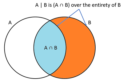
In a nutshell, conditional probability is to gain in information about an event that leads to a change in its probability. Suppose an event happens with probability . However, when event happens, this influences the probability of such that we have as the conditional probability of happening given occurred. Mathematically we know this as:
Figure 1 shows a Venn diagram that can visualize this. The is the relative probability of event happening with respect to event happening. Therefore, it justifies that we first need to get then dividing this by . It's just a matter of shifting the scope of event happening with respect to the entire space to the scope of event happening with respect to the space of event . We can rearrange the equation to get:
We can extend this concept to three or more sets. For example, if , , and are some events in a sample space, then we can compute the intersection of all events as:
Here's another interesting formula: Suppose we have a partition set of some sample space with each . In other words, we just cut the sample space into several partitions. Let event . In other words, event is just a part of the partition . We have:
Figure 2 visualizes this formula. The entire space is and we cut it into several components. Suppose event is also part of the entire space , then it's simply the sum of all components. You might wonder why the summation is from up to when we could just get the probabilities where it only matters? You are correct to think that we only need to get those that have a contribution to but the equation is generalized to include all partitions. For example, because event and event can never happen. So it's okay to generalize the formula to include all events even when their intersections don't happen at all.
Bayes' Theorem
Bayes' theorem is an extension of the conditional probability. Consider again that we have events and of some sample space . Bayes' theorem states that:
We can rearrange it to be aesthetically symmetric:
Bayes' theorem can be very useful to describe the probability of an event that is based on prior knowledge of conditions that may be related to the event.
Independence
In ordinary language, independence usually means that two experiences are completely separate. If an event happens it has no effect on the other. Given events and are independent, then the following should hold true:
Random Variables
A discrete random variable is a variable whose value is uncertain. In practice this random variable is just a mapping of different outcomes and their respective probabilities of occurring associated to a single variable only. We usually denote random variables with capital letters, just like . For example, let a discrete random variable represent the scenarios the sum of two independent die rolls. The set of possible outcomes would be:
Now, each outcome would have some probability associated with it. The list below shows the pair-wise mapping. We'll leave it as an exercise for you to determine how to get these probabilities.
The mapping between the outcomes and their corresponding probabilities is called a probability distribution. It describes the chances of the random variable to be one of the outcomes. It is common to visualize discrete random variables with bar graphs. Figure 3 shows the probability distribution of our two die rolls example.


