Difference between revisions of "Passive Matching Networks"
| (155 intermediate revisions by the same user not shown) | |||
| Line 1: | Line 1: | ||
| − | Controlling impedances in RF circuits | + | Controlling impedances in radio-frequency (RF) circuits is essential in order to maximize power transfer between blocks and to reduce reflections caused by impedance discontinuities along a signal path. In this module, we will define the quality factor, <math>Q</math>, for a device or a circuit, and use this <math>Q</math> to build circuits that modify the impedance seen across a port. |
== Device Quality Factor == | == Device Quality Factor == | ||
| − | The quality factor, Q, is a measure of how good a device is at storing energy. Thus, the lower the losses, the higher the Q. In general, if we can express the impedance or admittance of a device as | + | The quality factor, <math>Q</math>, is a measure of how good a device is at storing energy. Thus, the lower the losses, the higher the <math>Q</math>. In general, if we can express the impedance or admittance of a device as |
{{NumBlk|::|<math>Y\,\mathrm{or}\,Z=\frac{1}{A + jB}</math>|{{EquationRef|1}}}} | {{NumBlk|::|<math>Y\,\mathrm{or}\,Z=\frac{1}{A + jB}</math>|{{EquationRef|1}}}} | ||
| Line 13: | Line 13: | ||
=== Series RC Circuit === | === Series RC Circuit === | ||
| − | A lossy capacitor can be modeled as a series RC circuit with the series resistance, <math>R_S</math>, could represent the series loss due to interconnect resistances. Thus, the admittance of the lossy capacitor can be expressed as | + | [[File:RC Qseries.png|thumb|400px|Figure 1: A lossy capacitor.]] |
| + | |||
| + | A lossy capacitor, shown in Fig. 1, can be modeled as a series RC circuit with the series resistance, <math>R_S</math>, could represent the series loss due to interconnect resistances. Thus, the admittance of the lossy capacitor can be expressed as | ||
{{NumBlk|::|<math>Y_S =\frac{1}{R_S+\frac{1}{j\omega C}}</math>|{{EquationRef|3}}}} | {{NumBlk|::|<math>Y_S =\frac{1}{R_S+\frac{1}{j\omega C}}</math>|{{EquationRef|3}}}} | ||
| Line 19: | Line 21: | ||
We can therefore express the quality factor of the series circuit as: | We can therefore express the quality factor of the series circuit as: | ||
| − | {{NumBlk|::|<math>Q_S = \frac{\frac{1}{\omega C}}{R_S}=\frac{1}{\omega R_S C}</math>|{{EquationRef|4}}}} | + | {{NumBlk|::|<math>Q_S = \frac{\frac{1}{\omega C}}{R_S}=\frac{1}{\omega R_S C} = \frac{X_S}{R_S}</math>|{{EquationRef|4}}}} |
| − | Note that for the lossless case, <math>R_S=0</math>, | + | Note that for the lossless case, <math>R_S=0</math>, and consequently <math>Q_{S,\mathrm{ideal}} \rightarrow \infty</math>. |
=== Parallel RC Circuit === | === Parallel RC Circuit === | ||
| Line 30: | Line 32: | ||
Thus, the quality factor is: | Thus, the quality factor is: | ||
| − | {{NumBlk|::|<math>Q_P = \frac{\omega C}{\frac{1}{R_P}}=\omega R_P C</math>|{{EquationRef|6}}}} | + | {{NumBlk|::|<math>Q_P = \frac{\omega C}{\frac{1}{R_P}}=\omega R_P C=\frac{R_P}{X_P}</math>|{{EquationRef|6}}}} |
| − | We can see that in the lossless case, <math>R_P \rightarrow \infty</math>, | + | We can see that in the lossless case, <math>R_P \rightarrow \infty</math>, corresponding to <math>Q_{P,\mathrm{ideal}} \rightarrow \infty</math>. |
=== RL Circuits === | === RL Circuits === | ||
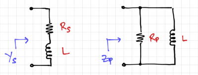
| − | Applying the ideas above to RL circuits, we can get the admittance of a series RL circuit as: | + | [[File:RL Qseries.png|thumb|400px|Figure 2: A lossy inductor.]] |
| + | |||
| + | Applying the ideas above to RL circuits in Fig. 2, we can get the admittance of a series RL circuit as: | ||
{{NumBlk|::|<math>Y_S =\frac{1}{R_S+j\omega L}</math>|{{EquationRef|7}}}} | {{NumBlk|::|<math>Y_S =\frac{1}{R_S+j\omega L}</math>|{{EquationRef|7}}}} | ||
| Line 41: | Line 45: | ||
with quality factor: | with quality factor: | ||
| − | {{NumBlk|::|<math>Q_S = \frac{\omega L}{R_S}</math>|{{EquationRef|8}}}} | + | {{NumBlk|::|<math>Q_S = \frac{\omega L}{R_S}=\frac{X_S}{R_S}</math>|{{EquationRef|8}}}} |
Similarly, for parallel RL circuits, the impedance and quality factor can be expressed as: | Similarly, for parallel RL circuits, the impedance and quality factor can be expressed as: | ||
| Line 47: | Line 51: | ||
{{NumBlk|::|<math>Z_P =\frac{1}{\frac{1}{R_P}+\frac{1}{j\omega L}}</math>|{{EquationRef|9}}}} | {{NumBlk|::|<math>Z_P =\frac{1}{\frac{1}{R_P}+\frac{1}{j\omega L}}</math>|{{EquationRef|9}}}} | ||
| − | {{NumBlk|::|<math>Q_P = \frac{\frac{1}{\omega L}}{\frac{1}{R_P}}=\frac{R_P}{\omega L}</math>|{{EquationRef|10}}}} | + | {{NumBlk|::|<math>Q_P = \frac{\frac{1}{\omega L}}{\frac{1}{R_P}}=\frac{R_P}{\omega L} = \frac{R_P}{X_P}</math>|{{EquationRef|10}}}} |
| + | |||
| + | Note that the quality factor is frequency dependent, and for <math>R_S=0</math> or <math>R_P \rightarrow \infty</math>, we get the ideal case where <math>Q_{S,\mathrm{ideal}} \rightarrow \infty</math> or <math>Q_{P,\mathrm{ideal}} \rightarrow \infty</math> respectively. | ||
| + | |||
| + | === General Case === | ||
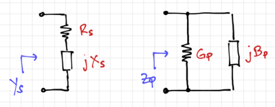
| + | [[File:Generic Qseries.png|thumb|400px|Figure 3: A lossy reactance.]] | ||
| + | |||
| + | In general, for a reactance <math>X_S</math> in series with a resistance <math>R_S</math>, | ||
| + | |||
| + | {{NumBlk|::|<math>Y_S =\frac{1}{R_S+jX_S}</math>|{{EquationRef|11}}}} | ||
| + | |||
| + | {{NumBlk|::|<math>Q_S = \frac{X_S}{R_S}</math>|{{EquationRef|12}}}} | ||
| + | |||
| + | and for a reactance <math>X_P = \tfrac{1}{B_P}</math> in parallel with a resistance <math>R_P = \tfrac{1}{G_P}</math>, | ||
| + | |||
| + | {{NumBlk|::|<math>Z_P =\frac{1}{G_P + jB_P}</math>|{{EquationRef|13}}}} | ||
| − | + | {{NumBlk|::|<math>Q_P = \frac{B_P}{G_P}= \frac{R_P}{X_P}</math>|{{EquationRef|14}}}} | |
== Series-Parallel Conversions == | == Series-Parallel Conversions == | ||
| − | It is very convenient to be able to convert the series RC or RL circuit to its parallel equivalent or vice-versa, especially in the context of matching circuits. | + | It is very convenient to be able to convert the series RC or RL circuit to its parallel equivalent or vice-versa, especially in the context of matching circuits. If we equate the parallel and series impedances, <math>\tfrac{1}{Y_S} = Z_S = Z_P</math>, we get |
| + | |||
| + | {{NumBlk|::|<math>R_S+ jX_S =\frac{1}{\frac{1}{R_P} + \frac{1}{jX_P}} = \frac{jR_P X_P}{R_P + jX_P}</math>|{{EquationRef|15}}}} | ||
| − | {{NumBlk|::|<math> | + | {{NumBlk|::|<math>\left(R_S+ jX_S\right)\left(R_P + jX_P \right) =jR_P X_P</math>|{{EquationRef|16}}}} |
| − | + | {{NumBlk|::|<math>R_S R_P + jR_P X_S+ jR_S X_P - X_S X_P = jR_P X_P</math>|{{EquationRef|17}}}} | |
| − | {{NumBlk|::|<math>\frac{ | + | We can look at the imaginary and real components separately. For the real components: |
| + | |||
| + | {{NumBlk|::|<math>R_S R_P - X_S X_P = 0</math>|{{EquationRef|18}}}} | ||
| + | |||
| + | {{NumBlk|::|<math>\frac{R_P}{X_P} = Q_P = \frac{X_S}{R_S} = Q_S = Q</math>|{{EquationRef|19}}}} | ||
| + | |||
| + | And for the imaginary components: | ||
| + | |||
| + | {{NumBlk|::|<math>R_P X_S + R_S X_P = R_P X_P</math>|{{EquationRef|20}}}} | ||
| + | |||
| + | Using eq. 18 and eq. 20, we get: | ||
| + | |||
| + | {{NumBlk|::|<math>\frac{X_S X_P}{R_S} X_S + R_S X_P = R_P X_P</math>|{{EquationRef|21}}}} | ||
| + | |||
| + | {{NumBlk|::|<math>\frac{X_S^2}{R_S^2} R_S + R_S = R_S\left(1 + Q^2\right)= R_P </math>|{{EquationRef|22}}}} | ||
| + | |||
| + | We can use eqs. 18 and 22 to get the relationship between the series and parallel reactances: | ||
| + | |||
| + | {{NumBlk|::|<math>R_S R_P - X_S X_P = R_S^2\left(1 + Q^2\right) - X_S X_P =0</math>|{{EquationRef|23}}}} | ||
| + | |||
| + | {{NumBlk|::|<math>R_S^2\left(1 + Q^2\right) - X_S X_P =R_S^2\left(1 + Q^2\right)\frac{X_S^2}{X_S^2} - X_S X_P = \frac{1 + Q^2}{Q^2} X_S - X_P = 0</math>|{{EquationRef|24}}}} | ||
| + | |||
| + | Rewriting eq. 24 and for <math>Q^2 \gg 1</math>: | ||
| + | |||
| + | {{NumBlk|::|<math>X_P = \frac{1 + Q^2}{Q^2} X_S = \left(1 + \frac{1}{Q^2}\right) X_S \approx X_S</math>|{{EquationRef|25}}}} | ||
| + | |||
| + | {{Note|'''Key Results''': | ||
| + | * The quality factor is the same for the parallel and series circuits when the impedances are the same. | ||
| + | |||
| + | {{NumBlk|::|<math>\frac{R_P}{X_P} = Q_P = \frac{X_S}{R_S} = Q_S = Q</math>|{{EquationRef|26}}}} | ||
| + | |||
| + | * The parallel resistance is larger than the series resistance. | ||
| + | {{NumBlk|::|<math>R_P = R_S\left(1 + Q^2\right)</math>|{{EquationRef|27}}}} | ||
| + | |||
| + | * The parallel reactance is approximately equal to the series reactance for <math>Q^2 \gg 1</math>. | ||
| + | {{NumBlk|::|<math>X_P = \left(1 + \frac{1}{Q^2}\right) X_S \approx X_S</math>|{{EquationRef|28}}}} | ||
| + | }} | ||
== Basic Matching Networks == | == Basic Matching Networks == | ||
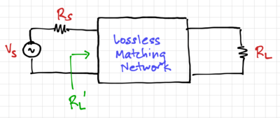
| + | [[File:Matching block diagram.png|thumb|400px|Figure 4: An impedance matching network.]] | ||
| + | We can use our series-parallel conversions to increase or decrease resistances based on the quality factor. Consider the circuit in Fig. 4, where we want to match the source resistance, <math>R_S</math> to a load resistance, <math>R_L</math> using a lossless matching network, i.e. a network make up of only reactances. | ||
| + | |||
| + | === L-Section Matching Circuits === | ||
| + | [[File:Matching L section.png|thumb|300px|Figure 5: An L-Section matching network and the network after the parallel-to-serial transformation of <math>R_L</math> and <math>jX_1</math>.]] | ||
| + | |||
| + | Consider the circuit in Fig. 5, and assume <math>R_S<R_L</math>. We can use our parallel-series transformations to convert the parallel circuit into a series circuit so that the the series resistance <math>R_L^\prime</math> is equivalent to the source resistance, <math>R_S</math> | ||
| + | |||
| + | {{NumBlk|::|<math>R_L^\prime = \frac{R_L}{1 + Q^2}</math>|{{EquationRef|29}}}} | ||
| + | |||
| + | Where <math>Q =\frac{R_L}{X_1}</math>. The reactance <math>X_1</math> also gets transformed into: | ||
| + | |||
| + | {{NumBlk|::|<math>X_1^\prime = X_1 \frac{1}{\left(1 + \frac{1}{Q^2}\right)} \approx X_1</math>|{{EquationRef|30}}}} | ||
| + | |||
| + | Thus, to keep the impedance seen by the source purely resistive, we can cancel out the reactance <math>X_1^\prime</math> by the reactance <math>X_2 = -X_1^\prime \approx -X_1</math>. Note that the negative sign relating <math>X_1</math> and <math>X_2</math> means that if <math>X_1</math> is a capacitance, then <math>X_2</math> should be an inductance, and vice-versa. Note that cancelling reactances at resonance could cause large voltages to appear across (or large currents through) the reactances. See this note on [[Resonance | resonance]] for more details. For the case when <math>R_S>R_L</math>, we just flip the circuit and the equations would still hold. | ||
| + | |||
| + | === Design Example === | ||
| + | Let define the ''matching factor'' <math>m =\tfrac{R_{\mathrm{hi}}}{R_{\mathrm{lo}}}</math>, where <math>R_\mathrm{hi}=\max\left(R_S, R_L\right)</math> and <math>R_\mathrm{lo}=\min\left(R_S, R_L\right)</math>. Therefore for <math>R_L>R_S</math>, <math>R_{\mathrm{hi}}=R_L</math> and <math>R_{\mathrm{lo}}=R_S</math>. We can then use eq. 29 to solve for the value of <math>Q</math>, <math>X_1</math>, and <math>X_1^\prime</math>: | ||
| + | |||
| + | {{NumBlk|::|<math>Q=\sqrt{m - 1} = \frac{R_L}{X_1}=\frac{X_1^\prime}{R_S}</math>|{{EquationRef|31}}}} | ||
| + | |||
| + | If we use a capacitor for <math>X_1</math>, then <math>C_1 = \tfrac{1}{\omega X_1}</math>. Thus, we need an inductance, <math>L_2=\tfrac{X_2}{\omega} =\tfrac{-X_1^\prime}{\omega}\approx \tfrac{-X_1}{\omega}</math>. Solving for <math>L_2</math>: | ||
| + | |||
| + | {{NumBlk|::|<math>L_2 = \frac{1}{\omega^2 C_1^\prime} \approx \frac{1}{\omega^2 C_1}</math>|{{EquationRef|32}}}} | ||
| + | |||
| + | Note that matching circuit is narrowband since the perfect cancellation occurs at only one frequency, <math>\omega</math>. | ||
| + | |||
| + | Instead of a capacitor, we can place an inductor in parallel with the larger resistance, and use a series capacitor to cancel out the series equivalent inductance. However, in this case, the capacitor will block any DC and low-frequency signals. | ||
== Loss in Matching Networks == | == Loss in Matching Networks == | ||
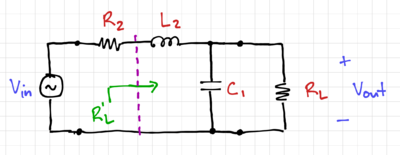
| + | [[File:Lossy L match.png|thumb|400px|Figure 6: A lossy L-section.]] | ||
| + | In typical real matching networks, the series resistance of the inductor is the dominant loss mechanism. We can model this loss using a resistor <math>R_2</math> in series with the inductor <math>L_2</math>, as shown in Fig. 6. | ||
| + | |||
| + | To determine the power loss due to <math>R_2</math>, we first calculate the power delivered by the input source: | ||
| + | |||
| + | {{NumBlk|::|<math>P_{\mathrm{in}} = \frac{V_{\mathrm{in}}^2}{R_2 + R_L^\prime}</math>|{{EquationRef|33}}}} | ||
| + | |||
| + | Then we calculate the power delivered to the load, <math>R_L</math>: | ||
| + | |||
| + | {{NumBlk|::|<math>P_L = \left(V_{\mathrm{in}} \frac{R_L^\prime}{R_2 + R_L^\prime}\right)^2 \frac{1}{R_L^\prime}</math>|{{EquationRef|34}}}} | ||
| + | |||
| + | We can then define power loss as | ||
| + | |||
| + | {{NumBlk|::|<math>\mathrm{Loss} = \frac{P_{\mathrm{in}}}{P_L}=\frac{R_2 + R_L^\prime}{R_L^\prime}=1 + \frac{R_2}{R_L^\prime}=1 + \frac{R_2\left(1 + Q^2\right)}{R_L}</math>|{{EquationRef|35}}}} | ||
| + | |||
| + | Note that the loss is dependent on the ratio of <math>R_2</math> to <math>R_L^\prime</math>. Thus, even if <math>R_2</math> is small, <math>R_L^\prime</math> can be relatively small as well, depending on the value of <math>Q</math>. In some cases, it is more convenient to use the inverse of eq. 35, or commonly known as ''Insertion Loss'' (IL): | ||
| + | |||
| + | {{NumBlk|::|<math>\mathrm{IL}=\frac{P_L}{P_\mathrm{in}}=\frac{1}{\mathrm{Loss}}</math>|{{EquationRef|36}}}} | ||
| + | |||
| + | If we define the inductor component quality factor as <math>Q_c = \tfrac{\omega L_2}{R_2}</math>, with <math>Q = \omega C_1 R_L =\tfrac{1}{\omega C_1^\prime R_L^\prime}</math> and <math>\omega^2 = \tfrac{1}{L_2 C_1^\prime}</math>, we can express the loss as: | ||
| + | |||
| + | {{NumBlk|::|<math>\mathrm{Loss} = 1 + \frac{R_2}{R_L^\prime} = 1 + \frac{\frac{\omega L_2}{Q_c}}{\frac{1}{\omega C_1^\prime Q}}=1 + \frac{Q}{Q_c}</math>|{{EquationRef|37}}}} | ||
| + | |||
| + | == T- and <math>\Pi</math>-Matching Networks == | ||
| + | [[File:Pi match.png|thumb|400px|Figure 7: A <math>\Pi</math>-matching network.]] | ||
| + | |||
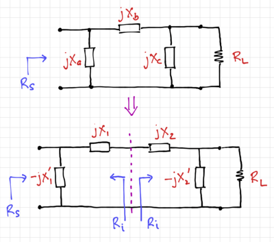
| + | Single L-section matching circuits are simple and elegant. However, we cannot choose the value of <math>Q</math> since it is determined by <math>m = \tfrac{R_\mathrm{hi}}{R_\mathrm{lo}}</math>. One way to increase the value of <math>Q</math> is to use two L-sections and an low intermediate resistance, <math>R_i</math>, where <math>R_i<R_S</math> and <math>R_i<R_L</math>, as shown in the <math>\Pi</math>-network in Fig. 7. | ||
| + | |||
| + | The first L-section reduces the value of source resistance, <math>R_S</math>, to the intermediate resistance, <math>R_i</math>, and the second L-section brings resistance from <math>R_i</math> to <math>R_L</math>. | ||
| + | |||
| + | We can then compute the quality factor of the two L-sections as: | ||
| + | |||
| + | {{NumBlk|::|<math>Q_1 = \sqrt{\frac{R_S}{R_i} - 1} = \frac{X_1}{R_i}=\frac{R_S}{X_1^\prime}</math>|{{EquationRef|38}}}} | ||
| + | |||
| + | {{NumBlk|::|<math>Q_2 = \sqrt{\frac{R_L}{R_i} - 1} = \frac{X_2}{R_i}=\frac{R_L}{X_2^\prime}</math>|{{EquationRef|39}}}} | ||
| + | |||
| + | [[File:Pi match Q.png|thumb|400px|Figure 8: Calculating the overall <math>Q</math> of a <math>\Pi</math>-network.]] | ||
| + | |||
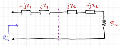
| + | From Fig. 8, the overall <math>Q</math> can be calculated by converting the parallel circuits into their series equivalents. Therefore: | ||
| + | |||
| + | {{NumBlk|::|<math>Q = \frac{X_1 + X_2}{2R_i} = \frac{Q_1 + Q_2}{2}</math>|{{EquationRef|40}}}} | ||
| + | |||
| + | [[File:T match.png|thumb|400px|Figure 9: A T-matching network.]] | ||
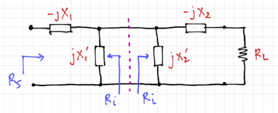
| + | If we want an intermediate resistance, <math>R_i</math>, that is larger than both <math>R_S</math> and <math>R_L</math>, we can use a T-network instead of a <math>\Pi</math>-network, as shown in Fig. 9. | ||
| + | |||
| + | In this case, | ||
| + | |||
| + | {{NumBlk|::|<math>Q_1 = \sqrt{\frac{R_i}{R_S} - 1} = \frac{R_i}{X_1^\prime}=\frac{X_1}{R_S}</math>|{{EquationRef|41}}}} | ||
| + | |||
| + | {{NumBlk|::|<math>Q_2 = \sqrt{\frac{R_i}{R_L} - 1} = \frac{R_i}{X_2^\prime}=\frac{X_2}{R_L}</math>|{{EquationRef|42}}}} | ||
| + | |||
| + | Similar to the <math>\Pi</math>-network, the overall T-network quality factor is <math>Q=\tfrac{1}{2}\left(Q_1 + Q_2\right)</math>. | ||
| + | |||
| + | == Multi-Section Low-<math>Q</math> Matching == | ||
| + | [[File:LowQ match.png|thumb|400px|Figure 10: A low-<math>Q</math> cascaded-L matching network.]] | ||
| + | |||
| + | T- and <math>\Pi</math>-networks are used to increase the overall <math>Q</math>. However, in some applications, a lower <math>Q</math> is required, especially in broadband circuits. Low <math>Q</math> circuits are also more robust to process variations and have relatively lower losses. To lower the quality factor of a matching network, we can cascade L-sections with an intermediate resistance, <math>R_\mathrm{hi}>R_i>R_\mathrm{lo}</math>, as shown in Fig. 10 for <math>R_S<R_L</math>. | ||
| + | |||
| + | The quality factor can be expressed as | ||
| + | |||
| + | {{NumBlk|::|<math>Q = \frac{1}{2}\left(Q_1 + Q_2\right) =\frac{1}{2}\left(\sqrt{\frac{R_i}{R_S} - 1} + \sqrt{\frac{R_L}{R_i} - 1}\right)</math>|{{EquationRef|43}}}} | ||
| + | |||
| + | To get the minimum possible <math>Q</math>, we can take the derivative of eq. 43 with respect to <math>R_i</math> and equate it to zero. This results in the optimum intermediate resistance: | ||
| + | |||
| + | {{NumBlk|::|<math>R_{i,\mathrm{opt}} = \sqrt{R_S R_L}</math>|{{EquationRef|44}}}} | ||
| + | |||
| + | Which leads to the minimum quality factor for two cascaded L-sections: | ||
| + | |||
| + | {{NumBlk|::|<math>Q_\min = \sqrt{\sqrt{\frac{R_S}{R_L}} - 1}</math>|{{EquationRef|45}}}} | ||
| − | + | {{Note|[[229-A1.2 | '''Activity A1.2''' Passive Matching Networks]] -- This activity walks you through the steps in designing and simulating passive matching networks.|reminder}} | |
Latest revision as of 14:36, 16 September 2020
Controlling impedances in radio-frequency (RF) circuits is essential in order to maximize power transfer between blocks and to reduce reflections caused by impedance discontinuities along a signal path. In this module, we will define the quality factor, , for a device or a circuit, and use this to build circuits that modify the impedance seen across a port.
Contents
Device Quality Factor
The quality factor, , is a measure of how good a device is at storing energy. Thus, the lower the losses, the higher the . In general, if we can express the impedance or admittance of a device as
-
(1)
-
The quality factor can then be expressed as
-
(2)
-
The imaginary component, represents the energy storage element, and the real component, , represents the loss (resistive) component.
Series RC Circuit
A lossy capacitor, shown in Fig. 1, can be modeled as a series RC circuit with the series resistance, , could represent the series loss due to interconnect resistances. Thus, the admittance of the lossy capacitor can be expressed as
-
(3)
-
We can therefore express the quality factor of the series circuit as:
-
(4)
-
Note that for the lossless case, , and consequently .
Parallel RC Circuit
A lossy capacitor can also be modeled as a parallel RC circuit, with the parallel resistance, could represent the energy loss due to the dielectric leakage of the capacitor. In this case, we can write the impedance of the circuit as:
-
(5)
-
Thus, the quality factor is:
-
(6)
-
We can see that in the lossless case, , corresponding to .
RL Circuits
Applying the ideas above to RL circuits in Fig. 2, we can get the admittance of a series RL circuit as:
-
(7)
-
with quality factor:
-
(8)
-
Similarly, for parallel RL circuits, the impedance and quality factor can be expressed as:
-
(9)
-
-
(10)
-
Note that the quality factor is frequency dependent, and for or , we get the ideal case where or respectively.
General Case
In general, for a reactance in series with a resistance ,
-
(11)
-
-
(12)
-
and for a reactance in parallel with a resistance ,
-
(13)
-
-
(14)
-
Series-Parallel Conversions
It is very convenient to be able to convert the series RC or RL circuit to its parallel equivalent or vice-versa, especially in the context of matching circuits. If we equate the parallel and series impedances, , we get
-
(15)
-
-
(16)
-
-
(17)
-
We can look at the imaginary and real components separately. For the real components:
-
(18)
-
-
(19)
-
And for the imaginary components:
-
(20)
-
Using eq. 18 and eq. 20, we get:
-
(21)
-
-
(22)
-
We can use eqs. 18 and 22 to get the relationship between the series and parallel reactances:
-
(23)
-
-
(24)
-
Rewriting eq. 24 and for :
-
(25)
-
- The quality factor is the same for the parallel and series circuits when the impedances are the same.
-
(26)
-
- The parallel resistance is larger than the series resistance.
-
(27)
-
- The parallel reactance is approximately equal to the series reactance for .
-
(28)
-
Basic Matching Networks
We can use our series-parallel conversions to increase or decrease resistances based on the quality factor. Consider the circuit in Fig. 4, where we want to match the source resistance, to a load resistance, using a lossless matching network, i.e. a network make up of only reactances.
L-Section Matching Circuits
Consider the circuit in Fig. 5, and assume . We can use our parallel-series transformations to convert the parallel circuit into a series circuit so that the the series resistance is equivalent to the source resistance,
-
(29)
-
Where . The reactance also gets transformed into:
-
(30)
-
Thus, to keep the impedance seen by the source purely resistive, we can cancel out the reactance by the reactance . Note that the negative sign relating and means that if is a capacitance, then should be an inductance, and vice-versa. Note that cancelling reactances at resonance could cause large voltages to appear across (or large currents through) the reactances. See this note on resonance for more details. For the case when , we just flip the circuit and the equations would still hold.
Design Example
Let define the matching factor , where and . Therefore for , and . We can then use eq. 29 to solve for the value of , , and :
-
(31)
-
If we use a capacitor for , then . Thus, we need an inductance, . Solving for :
-
(32)
-
Note that matching circuit is narrowband since the perfect cancellation occurs at only one frequency, .
Instead of a capacitor, we can place an inductor in parallel with the larger resistance, and use a series capacitor to cancel out the series equivalent inductance. However, in this case, the capacitor will block any DC and low-frequency signals.
Loss in Matching Networks
In typical real matching networks, the series resistance of the inductor is the dominant loss mechanism. We can model this loss using a resistor in series with the inductor , as shown in Fig. 6.
To determine the power loss due to , we first calculate the power delivered by the input source:
-
(33)
-
Then we calculate the power delivered to the load, :
-
(34)
-
We can then define power loss as
-
(35)
-
Note that the loss is dependent on the ratio of to . Thus, even if is small, can be relatively small as well, depending on the value of . In some cases, it is more convenient to use the inverse of eq. 35, or commonly known as Insertion Loss (IL):
-
(36)
-
If we define the inductor component quality factor as , with and , we can express the loss as:
-
(37)
-
T- and -Matching Networks
Single L-section matching circuits are simple and elegant. However, we cannot choose the value of since it is determined by . One way to increase the value of is to use two L-sections and an low intermediate resistance, , where and , as shown in the -network in Fig. 7.
The first L-section reduces the value of source resistance, , to the intermediate resistance, , and the second L-section brings resistance from to .
We can then compute the quality factor of the two L-sections as:
-
(38)
-
-
(39)
-
From Fig. 8, the overall can be calculated by converting the parallel circuits into their series equivalents. Therefore:
-
(40)
-
If we want an intermediate resistance, , that is larger than both and , we can use a T-network instead of a -network, as shown in Fig. 9.
In this case,
-
(41)
-
-
(42)
-
Similar to the -network, the overall T-network quality factor is .
Multi-Section Low- Matching
T- and -networks are used to increase the overall . However, in some applications, a lower is required, especially in broadband circuits. Low circuits are also more robust to process variations and have relatively lower losses. To lower the quality factor of a matching network, we can cascade L-sections with an intermediate resistance, , as shown in Fig. 10 for .
The quality factor can be expressed as
-
(43)
-
To get the minimum possible , we can take the derivative of eq. 43 with respect to and equate it to zero. This results in the optimum intermediate resistance:
-
(44)
-
Which leads to the minimum quality factor for two cascaded L-sections:
-
(45)
-


