Difference between revisions of "Quality Factor"
| (3 intermediate revisions by the same user not shown) | |||
| Line 15: | Line 15: | ||
=== Example: A Lossy Inductor === | === Example: A Lossy Inductor === | ||
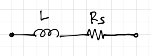
| + | [[File:Lossy L.png|thumb|300px|Figure 1: A lossy inductor.]] | ||
| + | [[File:Lossy C.png|thumb|300px|Figure 2: A lossy capacitor.]] | ||
For a lossy inductor, modeled as an ideal inductor with a series resistance, <math>R_s</math>, as shown in Fig. 1, we can write the admittance as: | For a lossy inductor, modeled as an ideal inductor with a series resistance, <math>R_s</math>, as shown in Fig. 1, we can write the admittance as: | ||
| Line 50: | Line 52: | ||
Where <math>\omega_p</math> is the distance of the pole from the origin, and <math>\sigma_x</math> is the distance of the pole from the <math>j\omega</math>-axis. This means that higher Q poles are closer to the <math>j\omega</math>-axis. | Where <math>\omega_p</math> is the distance of the pole from the origin, and <math>\sigma_x</math> is the distance of the pole from the <math>j\omega</math>-axis. This means that higher Q poles are closer to the <math>j\omega</math>-axis. | ||
| − | |||
| − | |||
| − | |||
| − | |||
| − | |||
== Band-Pass Filter Quality Factor == | == Band-Pass Filter Quality Factor == | ||
| Line 64: | Line 61: | ||
Where <math>\omega_c</math> is the center filter frequency, and <math>\Delta \omega = \omega_2 - \omega_1</math> is the filter bandwidth, as shown in Fig. 4. | Where <math>\omega_c</math> is the center filter frequency, and <math>\Delta \omega = \omega_2 - \omega_1</math> is the filter bandwidth, as shown in Fig. 4. | ||
| + | |||
| + | {| | ||
| + | |[[File:Pole Q.svg|thumb|300px|Figure 3: The pole quality factor.]] | ||
| + | |[[File:Bp filter Q.svg|thumb|400px|Figure 4: The band-pass filter quality factor.]] | ||
| + | |- | ||
| + | |} | ||
Latest revision as of 20:51, 16 March 2021
Let us review the many definitions of the quality factor, . This context-dependent metric can allow us to gain important insights on the behavior and implementation of energy storage and loss in circuits.
Contents
Component Quality Factor
For a transfer function that we can write as:
-
(1)
-
We can define the component quality factor, , as:
-
(2)
-
Example: A Lossy Inductor
For a lossy inductor, modeled as an ideal inductor with a series resistance, , as shown in Fig. 1, we can write the admittance as:
-
(3)
-
The quality factor of the lossy inductor is then equal to:
-
(4)
-
Example: A Lossy Capacitor
For a lossy capacitor, modeled as an ideal capacitor in parallel with a resistance, , as shown in Fig. 2, we can write the impedance as:
-
(5)
-
The quality factor of the lossy capacitor is then equal to:
-
(6)
-
Pole Quality Factor
The quality factor of a pole is a good indicator of the "cost" of implementing a pole. Higher Q poles have more stringent requirements in terms of loss, thus the pole Q allows us to determine which poles require more resources to implement.
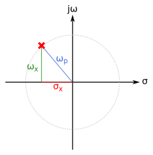
Consider the pole shown in Fig. 3. We define the pole quality factor as:
-
(7)
-
Where is the distance of the pole from the origin, and is the distance of the pole from the -axis. This means that higher Q poles are closer to the -axis.
Band-Pass Filter Quality Factor
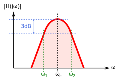
The band-pass filter quality factor, is a measure of the filter's bandwidth. The higher the quality factor, the more selectivity we have, and hence, lower loss is required to implement the filter. Thus, the band-pass filter quality factor is defined as:
-
(8)
-
Where is the center filter frequency, and is the filter bandwidth, as shown in Fig. 4.


