Difference between revisions of "Frequency Response Visualization"
Jump to navigation
Jump to search
| (2 intermediate revisions by the same user not shown) | |||
| Line 1: | Line 1: | ||
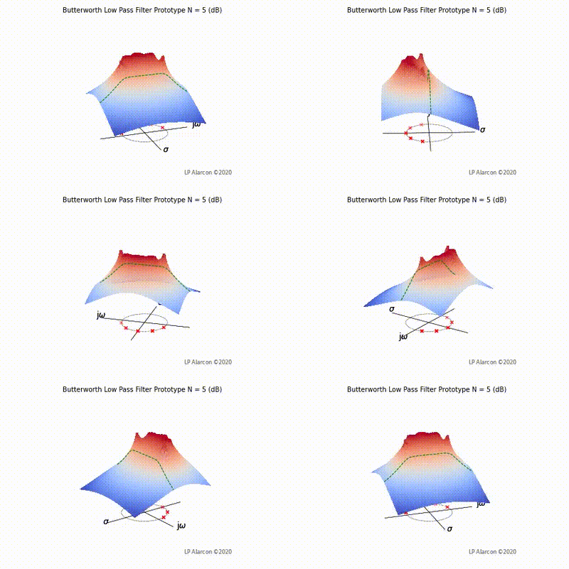
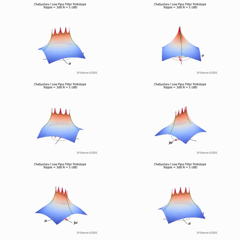
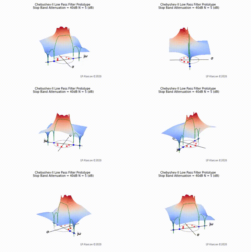
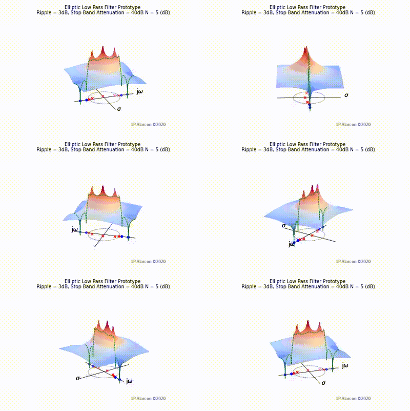
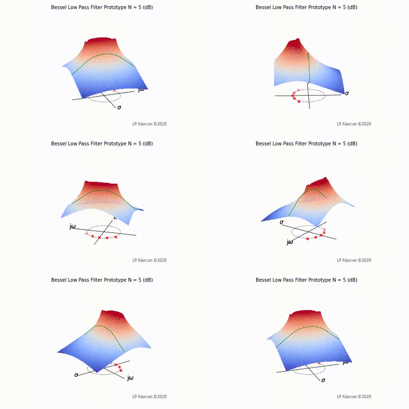
| − | The magnitude response of a linear system is the intersection of the magnitude of the transfer function, <math>\left|H\left(s\right)\right|</math>, in the <math>s=\sigma + j\omega</math> | + | The magnitude response of a linear system is the intersection of the magnitude of the transfer function, <math>\left|H\left(s\right)\right|</math>, in the <math>s=\sigma + j\omega</math> plane and the plane containing the <math>j\omega</math>-axis, as shown by the dashed green lines in Figs. 1-4. Note that the poles are the values of <math>s</math> that makes <math>\left|H\left(s\right)\right|\rightarrow\infty</math>, and the zeros are values of <math>s</math> that result in <math>\left|H\left(s\right)\right|=0</math>. |
{| | {| | ||
| Line 6: | Line 6: | ||
|- | |- | ||
|[[File:Chebyshev2 vid.gif|thumb|400px|Figure 3: The low-pass Chebyshev Type-II filter frequency response.]] | |[[File:Chebyshev2 vid.gif|thumb|400px|Figure 3: The low-pass Chebyshev Type-II filter frequency response.]] | ||
| − | |[[File:Elliptic vid.gif|thumb|400px|Figure | + | |[[File:Elliptic vid.gif|thumb|400px|Figure 4: The low-pass Elliptic filter frequency response.]] |
|- | |- | ||
| − | |[[File:Bessel vid.gif|thumb|400px|Figure | + | |[[File:Bessel vid.gif|thumb|400px|Figure 5: The low-pass Bessel filter frequency response.]] |
| | | | ||
|- | |- | ||
|} | |} | ||
Latest revision as of 00:21, 19 March 2021
The magnitude response of a linear system is the intersection of the magnitude of the transfer function, , in the plane and the plane containing the -axis, as shown by the dashed green lines in Figs. 1-4. Note that the poles are the values of that makes , and the zeros are values of that result in .


