Difference between revisions of "161-A2.1"
| (17 intermediate revisions by the same user not shown) | |||
| Line 104: | Line 104: | ||
{| | {| | ||
| − | |[[File:Code3 coding tree.png|400px|Fig. 3: A binary tree for code 3.]] | + | |[[File:Code3 coding tree.png|thumb|400px|Fig. 3: A binary tree for code 3.]] |
| − | |[[File:Code4 coding tree.png|400px|Fig. 4: A binary tree for code 4.]] | + | |[[File:Code4 coding tree.png|thumb|400px|Fig. 4: A binary tree for code 4.]] |
|- | |- | ||
|} | |} | ||
== Example 4: Huffman Coding == | == Example 4: Huffman Coding == | ||
| + | Huffman codes are an optimal variable-length prefix code, commonly used for lossless data compression. The algorithm for generating these codes was developed by David Huffman, and was published in his 1952 paper<ref>Huffman, D., ''A Method for the Construction of Minimum-Redundancy Codes''. Proceedings of the IRE. 40 (9): 1098–1101., September 1952, doi:10.1109/JRPROC.1952.273898 ([http://compression.ru/download/articles/huff/huffman_1952_minimum-redundancy-codes.pdf pdf])</ref> when he was a graduate student at MIT. Similar to all our entropy-based codes, shorter codes are assigned to symbols with higher probabilities. | ||
| − | == Activity: | + | Read more about David Huffman in this short [http://www.huffmancoding.com/my-uncle/scientific-american article]<ref>Gary Stix, ''Encoding the “Neatness” of Ones and Zeroes'', Scientific American, September 1991, pp. 54, 58 ([http://www.huffmancoding.com/my-uncle/scientific-american html])</ref> that originally appeared in the September 1991 issue of Scientific American. |
| + | |||
| + | === Coding the Source === | ||
| + | Given a source with alphabet <math>A=\{a_1, a_2, a_3, a_4, a_5\}</math>, with probabilities <math>P = \{0.15, 0.2, 0.25, 0.25, 0.15\}</math>, generate a Huffman code for this source. | ||
| + | |||
| + | The first step is to sort the symbols according to their probabilities, as shown in Fig. 5. We then choose the two symbols with the lowest probabilities (<math>a_1</math>) and (<math>a_5</math>), and replace them with a new symbol, whose probability is <math>0.15 + 0.15 = 0.3</math>. The symbols, including the new symbol that replaces <math>a_1</math> and <math>a_5</math>, are then sorted once again. We repeat this process until we combine all the symbols into one symbol with probability equal to 1. | ||
| + | |||
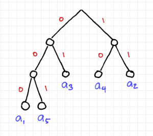
| + | Working backwards from the root of our tree, we can assign a '0' to the top fork, and a '1' to the bottom fork until we get to the original symbols. Fig. 6 shows the redrawn Huffman tree showing the codewords at the endpoints of the tree. | ||
| + | |||
| + | {| | ||
| + | |[[File:Huffman coding 1.png|thumb|500px|Figure 5: Huffman coding a source.]] | ||
| + | |[[File:Huffman tree 1.png|thumb|300px|Figure 6: The resulting Huffman tree.]] | ||
| + | |- | ||
| + | |} | ||
| + | |||
| + | This process results in the following codes: | ||
| + | |||
| + | {| class = "wikitable" | ||
| + | ! Symbol | ||
| + | ! <math>P</math> | ||
| + | ! Code | ||
| + | |- | ||
| + | | <math>a_1</math> | ||
| + | | 0.15 | ||
| + | | 000 | ||
| + | |- | ||
| + | | <math>a_2</math> | ||
| + | | 0.2 | ||
| + | | 11 | ||
| + | |- | ||
| + | | <math>a_3</math> | ||
| + | | 0.25 | ||
| + | | 01 | ||
| + | |- | ||
| + | | <math>a_4</math> | ||
| + | | 0.25 | ||
| + | | 10 | ||
| + | |- | ||
| + | | <math>a_5</math> | ||
| + | | 0.15 | ||
| + | | 001 | ||
| + | |- | ||
| + | |} | ||
| + | |||
| + | Notice that, as expected, the symbols with the highest probabilities are assigned shorter codewords. | ||
| + | |||
| + | === Evaluating the Code === | ||
| + | Let us check how good our Huffman code is. First, let us compute the entropy of the source: | ||
| + | |||
| + | {{NumBlk|::|<math>H\left(S\right) = 0.15\log_2\left(\frac{1}{0.15}\right) + 0.2\log_2\left(\frac{1}{0.2}\right) + 0.25\log_2\left(\frac{1}{0.25}\right) + 0.25\log_2\left(\frac{1}{0.25}\right) + 0.15\log_2\left(\frac{1}{0.15}\right) = 2.285\,\mathrm{bits}</math>|{{EquationRef|2}}}} | ||
| + | |||
| + | The average code length of our Huffman code is: | ||
| + | |||
| + | {{NumBlk|::|<math>L = 0.15\cdot 3 + 0.2\cdot 2 + 0.25\cdot 2 + 0.25\cdot 2 + 0.15\cdot 3 = 2.3\,\mathrm{bits}</math>|{{EquationRef|3}}}} | ||
| + | |||
| + | We can see that our Huffman code is very efficient, with the average length very close to the Shannon limit. | ||
| + | |||
| + | == Activity: Encode and Decode a File == | ||
| + | In this activity, you are to encode this text [https://github.com/louisalarcon/CoE161/blob/master/txt/ninoy_aquino_1983.txt file] using Huffman coding. You can do this activity by hand, but it will be very long and tedious. It is best to do this by writing your own program, preferably in a language that handles lists very well (e.g. Python). | ||
| + | |||
| + | You need to do the following steps: | ||
| + | # Determine the symbol or character probabilities. | ||
| + | # Calculate the entropy of the source, or in this case, the entropy of the text file. | ||
| + | # Create a Huffman tree and assign codes to each character or symbol. | ||
| + | # Encode the file using your generated Huffman code. | ||
| + | # Calculate the average codeword length of your code and compare it to the entropy of the file. | ||
| + | # Decode your encoded message, and verify that you do get the original message. | ||
| + | |||
| + | Please let me know if you encounter any difficulties or issues. I would be happy to help you out. | ||
| + | |||
| + | === Report Guide === | ||
| + | Write a 1-2 page report on your approach in performing this activity, showing: | ||
| + | * The details of how you implemented each of the steps outlined above including any visual aids such as flowcharts, images, pseudo-codes, etc. | ||
| + | * Comment on the codeword length vs. the symbol probability. Is this what you expected? | ||
| + | * Comment on the relative values of the source entropy and your average code length. | ||
| + | * Were you able to decode the message correctly? | ||
| + | * Compare your Huffman code to a file encoded using ASCII encoding. Comment on the length of the encoded file, and the decoding process. | ||
| + | |||
| + | === Submission === | ||
| + | Send your report via email before you start on Module 3. | ||
| + | |||
| + | == References == | ||
| + | <references /> | ||
Latest revision as of 16:46, 19 September 2020
- Activity: Source Coding
- Instructions: In this activity, you are tasked to
- Walk through the examples.
- Write a short program to compress and decompress a redundant file.
- Should you have any questions, clarifications, or issues, please contact your instructor as soon as possible.
Contents
Example 1: Uniquely Decodable Codes
Let us try to encode a source with just four symbols in its alphabet, i.e. , with probability distribution . We can calculate the entropy of this source as:
-
(1)
-
Let us look at a few bit sequence assignments and see if they are uniquely decodable or not.
| Symbol | Probability | Code 1 | Code 2 | Code 3 | Code 4 |
|---|---|---|---|---|---|
| 0.5 | 0 | 0 | 0 | 0 | |
| 0.25 | 0 | 1 | 10 | 01 | |
| 0.125 | 1 | 00 | 110 | 011 | |
| 0.125 | 10 | 11 | 111 | 0111 | |
| Average Code Length: | 1.125 | 1.25 | 1.75 | 1.875 | |
Recall that Shannon's Noiseless Coding Theorem states that . Thus, codes 1 and 2 are not uniquely decodable since they have average code lengths less than .
For code 1, since there are two symbols sharing an encoded symbol, we can say that it is not a distinct code, and therefore not uniquely decodable. We can check code 2 by taking a sequence of symbols encoded using this code: . We can easily see that this message can be decoded in different ways, either as , or .
Code 3 has one of the most desirable properties of a code: having its average length equal to the entropy of the source, and according to Shannon, you cannot have a uniquely decodable code with an average length shorter than this. We can also see that for a sequence of symbols encoded using code 3, there is only one way you can decode the message, thus it is uniquely decodable.
Code 4 is also uniquely decodable, however, it is not instantaneous, since the decoder needs to see the start of the next symbol to determine the end of the current symbol. Also note that the average length of code 4 is longer than the .
We can use the Kraft-McMillan Inequality, , to test if a code is uniquely decodable. Tabulating the values, we get:
| Code | |
|---|---|
| 1 | 1.75 |
| 2 | 1.5 |
| 3 | 1.0 |
| 4 | 0.9375 |
As expected, codes 1 and 2 have , and thus, are not uniquely decodable, while codes 3 and 4 have , and hence, they are uniquely decodable.
Example 2: Uniformly Distributed Symbols
Let us consider the case when the symbols are uniformly distributed, i.e. . We can then calculate the entropy of the source as:
-
(2)
-
In this case, the source is incompressible. Thus, we can just use a fixed length code .
Example 3: Prefix Codes
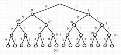
In prefix codes or prefix-free codes, no codeword is a proper prefix of another. One way to test this is to use trees. Fig. 1 shows a binary tree with 4 levels. This three can represent codewords with lengths of 1 to 4 bits. Thus, for a prefix code, all the codewords should only be at the leaves of the tree, or equivalently, at nodes without any codewords further down the tree.
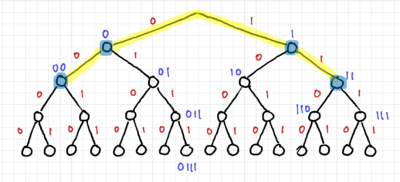
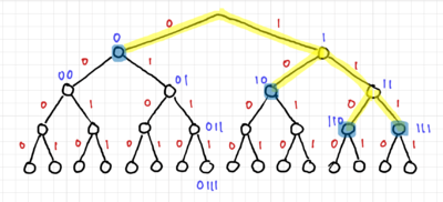
The tree for code 2 is shown in Fig. 2, and we can easily see that code 2 is not a prefix code since there are codewords within the tree. Fig. 3 shows the tree for code 3, and since all the codewords are at the edges of the tree, it is a prefix code, and thus uniquely decodable and instantaneous. Lastly, we have the tree for code 4 in Fig. 4, where only one of the codewords is at the edge of the tree. Thus, code 4 is not a prefix code.
Example 4: Huffman Coding
Huffman codes are an optimal variable-length prefix code, commonly used for lossless data compression. The algorithm for generating these codes was developed by David Huffman, and was published in his 1952 paper[1] when he was a graduate student at MIT. Similar to all our entropy-based codes, shorter codes are assigned to symbols with higher probabilities.
Read more about David Huffman in this short article[2] that originally appeared in the September 1991 issue of Scientific American.
Coding the Source
Given a source with alphabet , with probabilities , generate a Huffman code for this source.
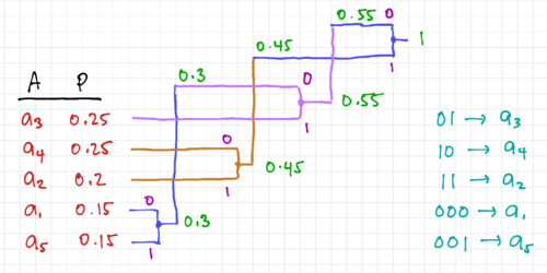
The first step is to sort the symbols according to their probabilities, as shown in Fig. 5. We then choose the two symbols with the lowest probabilities () and (), and replace them with a new symbol, whose probability is . The symbols, including the new symbol that replaces and , are then sorted once again. We repeat this process until we combine all the symbols into one symbol with probability equal to 1.
Working backwards from the root of our tree, we can assign a '0' to the top fork, and a '1' to the bottom fork until we get to the original symbols. Fig. 6 shows the redrawn Huffman tree showing the codewords at the endpoints of the tree.
This process results in the following codes:
| Symbol | Code | |
|---|---|---|
| 0.15 | 000 | |
| 0.2 | 11 | |
| 0.25 | 01 | |
| 0.25 | 10 | |
| 0.15 | 001 |
Notice that, as expected, the symbols with the highest probabilities are assigned shorter codewords.
Evaluating the Code
Let us check how good our Huffman code is. First, let us compute the entropy of the source:
-
(2)
-
The average code length of our Huffman code is:
-
(3)
-
We can see that our Huffman code is very efficient, with the average length very close to the Shannon limit.
Activity: Encode and Decode a File
In this activity, you are to encode this text file using Huffman coding. You can do this activity by hand, but it will be very long and tedious. It is best to do this by writing your own program, preferably in a language that handles lists very well (e.g. Python).
You need to do the following steps:
- Determine the symbol or character probabilities.
- Calculate the entropy of the source, or in this case, the entropy of the text file.
- Create a Huffman tree and assign codes to each character or symbol.
- Encode the file using your generated Huffman code.
- Calculate the average codeword length of your code and compare it to the entropy of the file.
- Decode your encoded message, and verify that you do get the original message.
Please let me know if you encounter any difficulties or issues. I would be happy to help you out.
Report Guide
Write a 1-2 page report on your approach in performing this activity, showing:
- The details of how you implemented each of the steps outlined above including any visual aids such as flowcharts, images, pseudo-codes, etc.
- Comment on the codeword length vs. the symbol probability. Is this what you expected?
- Comment on the relative values of the source entropy and your average code length.
- Were you able to decode the message correctly?
- Compare your Huffman code to a file encoded using ASCII encoding. Comment on the length of the encoded file, and the decoding process.
Submission
Send your report via email before you start on Module 3.


