The Data Processing Inequality

Entropy Chain Rule

Figure 1: Entropy visualization for two random variables using Venn diagrams.

As we increase the number of random variables we are dealing with, it is important to understand how this increase affects entropy. We have previously shown that for two random variables $X$ and $Y$:

${\begin{aligned}H\left(X,Y\right)&=H\left(X\right)+H\left(Y\mid X\right)\\&=H\left(Y\right)+H\left(X\mid Y\right)\\&=H\left(Y,X\right)\end{aligned}}$

(1)

We can use Venn diagrams to visualize these relationships, as seen in Fig. 1. For three random variables $X$, $Y$, and $Z$:

${\begin{aligned}H\left(X,Y,Z\right)&=H\left(X\right)+H\left(Y,Z\mid X\right)\\&=H\left(X\right)+H\left(Y\mid X\right)+H\left(Z\mid Y,X\right)\\\end{aligned}}$

(2)

In general:

$H\left(X_{1},X_{2},\ldots ,X_{n}\right)=\sum _{i=1}^{n}H\left(X_{i}\mid X_{i-1},X_{i-2},\ldots ,X_{1}\right)$

(3)

Conditional Mutual Information

Conditional mutual information is defined as the expected value of the mutual information of two random variables given the value of a third random variable, and for three random variables $X$, $Y$, and $Z$, it is defined as:

${\begin{aligned}I\left(X;Y\mid Z\right)&=\sum _{z\in Z}P\left(z\right)\sum _{y\in Y}\sum _{x\in X}P\left(x,y\mid z\right)\cdot \log _{2}{\frac {P\left(x,y\mid z\right)}{P\left(x\mid z\right)\cdot P\left(y\mid z\right)}}\\&=\sum _{z\in Z}\sum _{y\in Y}\sum _{x\in X}P\left(x,y,z\right)\cdot \log _{2}{\frac {P\left(x,y,z\right)\cdot P\left(z\right)}{P\left(x,z\right)\cdot P\left(y,z\right)}}\\\end{aligned}}$

(4)

We can rewrite the definition of conditional mutual information as:

${\begin{aligned}I\left(X;Y\mid Z\right)&=\sum _{z\in Z}\sum _{y\in Y}\sum _{x\in X}P\left(x,y,z\right)\cdot \log _{2}{\frac {P\left(x,y,z\right)\cdot P\left(z\right)}{P\left(x,z\right)\cdot P\left(y,z\right)}}\\&=\sum _{z\in Z}\sum _{y\in Y}\sum _{x\in X}P\left(x,y,z\right)\cdot \left(\log _{2}{\frac {P\left(z\right)}{P\left(x,z\right)}}-\log _{2}{\frac {P\left(y,z\right)}{P\left(x,y,z\right)}}\right)\\&=\sum _{z\in Z}\sum _{y\in Y}\sum _{x\in X}P\left(x,y,z\right)\cdot \log _{2}{\frac {P\left(z\right)}{P\left(x,z\right)}}-\sum _{z\in Z}\sum _{y\in Y}\sum _{x\in X}P\left(x,y,z\right)\cdot \log _{2}{\frac {P\left(y,z\right)}{P\left(x,y,z\right)}}\\&=\sum _{y\in Y}P\left(y\right)\sum _{z\in Z}\sum _{x\in X}P\left(x,z\mid y\right)\cdot \log _{2}{\frac {P\left(z\right)}{P\left(x,z\right)}}-\sum _{z\in Z}\sum _{y\in Y}\sum _{x\in X}P\left(x,y,z\right)\cdot \log _{2}{\frac {P\left(y,z\right)}{P\left(x,y,z\right)}}\\&=\sum _{z\in Z}\sum _{x\in X}P\left(x,z\right)\cdot \log _{2}{\frac {P\left(z\right)}{P\left(x,z\right)}}-\sum _{z\in Z}\sum _{y\in Y}\sum _{x\in X}P\left(x,y,z\right)\cdot \log _{2}{\frac {P\left(y,z\right)}{P\left(x,y,z\right)}}\\&=H\left(X\mid Z\right)-H\left(X\mid Y,Z\right)\\\end{aligned}}$

(5)

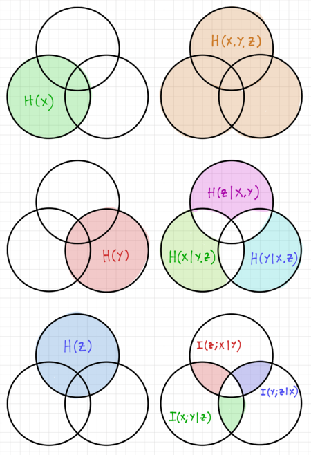
Figure 2: Entropy visualization for three random variables using Venn diagrams.

We can visualize this relationship using the Venn diagrams in Fig. 2. Compare this to our expression for the mutual information of two random variables $X$ and $Y$:

$I\left(X;Y\right)=H\left(X\right)-H\left(X\mid Y\right)$

(6)

Chain Rule for Mutual Information

For random variables $X$ and $Z$:

$I\left(X;Z\right)=H\left(X\right)-H\left(X\mid Z\right)$

(7)

And for random variables $X$, $Y$ and $Z$:

$I\left(X;Y,Z\right)=H\left(X\right)-H\left(X\mid Y,Z\right)$

(8)

We can then express the conditional mutual information as:

${\begin{aligned}I\left(X;Y\mid Z\right)&=H\left(X\mid Z\right)-H\left(X\mid Y,Z\right)\\&=H\left(X\right)-I\left(X;Z\right)+I\left(X;Y,Z\right)-H\left(X\right)\\&=I\left(X;Y,Z\right)-I\left(X;Z\right)\\\end{aligned}}$

(9)

Rearranging, we then obtain the chain rule for mutual information:

$I\left(X;Y,Z\right)=I\left(X;Y\mid Z\right)+I\left(X;Z\right)$

(10)

Thus, we can extend this for additional random variables:

${\begin{aligned}I\left(Y;X_{1},X_{2},X_{3}\right)&=I\left(Y;X_{3}\mid X_{2},X_{1}\right)+I\left(Y;X_{2},X_{1}\right)\\&=I\left(Y;X_{3}\mid X_{2},X_{1}\right)+I\left(Y;X_{2}\mid X_{1}\right)+I\left(Y;X_{1}\right)\\\end{aligned}}$

(11)

In general:

$I\left(Y;X_{1},X_{2},\ldots ,X_{n}\right)=\sum _{i=1}^{n}I\left(Y;X_{i}\mid X_{i-1},X_{i-2},\dots ,X_{1}\right)$

(12)

Markovity

A Markov Chain is a random process that describes a sequence of possible events where the probability of each event depends only on the outcome of the previous event. Thus, we say that $X,Y,Z$ is a Markov chain in this order, denoted as:

$X\rightarrow Y\rightarrow Z$

(13)

If we can write:

$P\left(X=x,Y=y,Z=z\right)=P\left(Z=z\mid Y=y\right)\cdot P\left(Y=y\mid X=x\right)\cdot P\left(X=x\right)$

(14)

Or in a more compact form:

$P\left(x,y,z\right)=P\left(z\mid y\right)\cdot P\left(y\mid x\right)\cdot P\left(x\right)$

(15)

We can use Markov chains to model how a signal is corrupted when passed through noisy channels. For example, if $X$ is a binary signal, it can change with a certain probability, $p$, to $Y$, and it can again be corrupted to produce $Z$.

Consider the joint probability $P\left(x,z\mid y\right)$. We can express this as:

$P\left(x,z\mid y\right)={\frac {P\left(x,y,z\right)}{P\left(y\right)}}$

(16)

And if $X\rightarrow Y\rightarrow Z$, we get:

$P\left(x,z\mid y\right)={\frac {P\left(z\mid y\right)\cdot P\left(y\mid x\right)\cdot P\left(x\right)}{P\left(y\right)}}$

(17)

Since $P\left(y,x\right)=P\left(y\mid x\right)\cdot P\left(x\right)=P\left(x\mid y\right)\cdot P\left(y\right)$, we can write:

$P\left(x,z\mid y\right)={\frac {P\left(z\mid y\right)\cdot P\left(y,x\right)}{P\left(y\right)}}=P\left(z\mid y\right)\cdot P\left(x\mid y\right)$

(18)

Thus, we can say that $X$ and $Z$ are conditionally independent given $Y$. If we think of $X$ as some past event, and $Z$ as some future event, then the past and future events are independent if we know the present event $Y$. Note that this property is good definition of, as well as a useful tool for checking Markovity.

We can rewrite the joint probability $P\left(x,y,z\right)$ as:

${\begin{aligned}P\left(x,y,z\right)&=P\left(z\mid y\right)\cdot P\left(y\mid x\right)\cdot P\left(x\right)\\&={\frac {P\left(z,y\right)}{P\left(y\right)}}\cdot P\left(y,x\right)\\&={\frac {P\left(z,y\right)}{P\left(y\right)}}\cdot P\left(x\mid y\right)\cdot P\left(y\right)\\&=P\left(z,y\right)\cdot P\left(x\mid y\right)\\&=P\left(x\mid y\right)\cdot P\left(y\mid z\right)\cdot P\left(z\right)\\\end{aligned}}$

(19)

Therefore, if $X\rightarrow Y\rightarrow Z$, then it follows that $Z\rightarrow Y\rightarrow X$.

The Data Processing Inequality

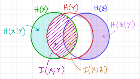
Figure 3: Venn diagram visualization of mutual information in a Markov chain.

Consider three random variables, $X$, $Y$, and $Z$. The mutual information $I\left(X;Y,Z\right)$ can be expressed as:

${\begin{aligned}I\left(X;Y,Z\right)&=I\left(X;Y\mid Z\right)+I\left(X;Z\right)\\&=I\left(X;Z\mid Y\right)+I\left(X;Y\right)\\\end{aligned}}$

(20)

If $X\rightarrow Y\rightarrow Z$, i.e. $X$, $Y$, and $Z$ form a Markov chain, then $X$ is conditionally independent of $Z$ given $Y$, resulting in $I\left(X;Z\mid Y\right)=0$. Thus,

${\begin{aligned}I\left(X;Y\mid Z\right)+I\left(X;Z\right)&=I\left(X;Z\mid Y\right)+I\left(X;Y\right)\\I\left(X;Y\mid Z\right)+I\left(X;Z\right)&=I\left(X;Y\right)\\\end{aligned}}$

(21)

And since $I\left(X;Y\mid Z\right)\geq 0$, we get the expression known as the Data Processing Inequality:

$I\left(X;Z\right)\leq I\left(X;Y\right)$

(21)

And since $Z\rightarrow Y\rightarrow X$ is also a Markov chain, then:

$I\left(Z;X\right)\leq I\left(Z;Y\right)$

(22)

We can visualize this relation using the Venn diagrams in Fig. 3. Note that the equality occurs when $I\left(X;Y\mid Z\right)=0$. It should also be evident that $X\mid Y$ is independent of $Z\mid Y$ given $Y$, and that $I\left(X;Z\mid Y\right)=0$.

Essentially, the data processing inequality implies that no amount of processing or clever manipulation of data can improve inference. Stated in another way, no clever transformation of the received code $Y$ can give more information about the sent code $X$. This implies that:

• We will loose information when we process information (downside).
• In some cases, the equality still holds even if we discard something (upside). This motivates our exploration of the concept of sufficient statistics.

Sufficient Statistics

Given a family of distributions $\{f_{\theta }\left(x\right)\}$ indexed by a parameter $\theta$. If $X$ is a sample from $f_{\theta }$, and $T\left(X\right)$ is any statistic, then we get the Markov chain:

$\theta \rightarrow X\rightarrow T\left(X\right)$

(23)

From the data processing inequality, we get:

$I\left(\theta ;T\left(X\right)\right)\leq I\left(\theta ;X\right)$

(24)

We say that a statistic is sufficient for $\theta$ if it has all the information contained in $X$ about $\theta$. Mathematically, this means:

$I\left(\theta ;T\left(X\right)\right)=I\left(\theta ;X\right)$

(25)

Or equivalently:

$\theta \rightarrow T\left(X\right)\rightarrow X$

(26)

That is, once we know $T\left(X\right)$, the remaining randomness in $X$ does not depend on $\theta$.

Fano's Inequality

Consider a communication system, where we transmit $X$, and receive the corrupted version $Y$. If we try to infer $X$ from $Y$, there is always a possibility that we will make a mistake. If ${\hat {X}}$ is our estimate of $X$, then $X\rightarrow Y\rightarrow {\hat {X}}$ is a Markov chain. We then define the probability of error as:

$P_{e}=P\left({\hat {X}}\neq X\right)$

(27)

Let us define the error random variable, $E$, as:

$E={\begin{cases}1,&\mathrm {if} \,{\hat {X}}\neq X\\0,&\mathrm {if} \,{\hat {X}}=X\\\end{cases}}$

(28)

We then get $H\left(E\right)=H\left(P_{e}\right)$. Using the entropy chain rule:

${\begin{aligned}H\left(X,Y\right)&=H\left(X\right)+H\left(Y\mid X\right)\\&=H\left(Y\right)+H\left(X\mid Y\right)\\\end{aligned}}$

(29)

Then the conditional entropy $H\left(E,X\mid {\hat {X}}\right)$ is:

${\begin{aligned}H\left(E,X\mid {\hat {X}}\right)&=H\left(E\mid {\hat {X}}\right)+H\left(X\mid E,{\hat {X}}\right)\\&=H\left(X\mid {\hat {X}}\right)+H\left(E\mid X,{\hat {X}}\right)\\\end{aligned}}$

(30)

Let us look at these terms one by one. If we know $X$ and ${\hat {X}}$, then there is no uncertainty in the value of $E$, thus:

$H\left(E\mid X,{\hat {X}}\right)=0$

(31)

Recall that conditioning reduces the uncertainty:

${\begin{aligned}H\left(E\mid {\hat {X}}\right)&=H\left(E\right)-I\left(E;{\hat {X}}\right)\\&\leq H\left(E\right)\\&\leq H\left(P_{e}\right)\\\end{aligned}}$

(32)

We can expand $H\left(X\mid E,{\hat {X}}\right)$ as:

$H\left(X\mid E,{\hat {X}}\right)=P\left(E=0\right)\cdot H\left(X\mid E=0,{\hat {X}}\right)+P\left(E=1\right)\cdot H\left(X\mid E=1,{\hat {X}}\right)$

(33)

Note that given $E=0$, i.e. there is no error, then there is no uncertainty in $X$ given ${\hat {X}}$, giving us $H\left(X\mid E=0,{\hat {X}}\right)=0$. And once again, we know conditioning reduces uncertainty, giving us $H\left(X\mid E=1,{\hat {X}}\right)\leq H\left(X\right)$. Thus, recognizing that $P\left(E=0\right)=1-P_{e}$ and $P\left(E=1\right)=P_{e}$, we get:

$H\left(X\mid E,{\hat {X}}\right)\leq P_{e}\cdot H\left(X\right)$

(34)

If both $X$ and ${\hat {X}}$ have symbols in the alphabet $\chi$, then applying the Gibbs inequality, we get $H\left(X\right)\leq \log _{2}\left|\chi \right|$, where $\left|\chi \right|$ is the number of symbols in $\chi$. This gives us:

$H\left(X\mid E,{\hat {X}}\right)\leq P_{e}\cdot \log _{2}\left|\chi \right|$

(35)

Combining these individual results, we can then write Eq. 30 as:

${\begin{aligned}H\left(E\mid {\hat {X}}\right)+H\left(X\mid E,{\hat {X}}\right)&=H\left(X\mid {\hat {X}}\right)+H\left(E\mid X,{\hat {X}}\right)\\H\left(P_{e}\right)+P_{e}\cdot \log _{2}\left|\chi \right|&\geq H\left(X\mid {\hat {X}}\right)\end{aligned}}$

(36)

Since $X\rightarrow Y\rightarrow {\hat {X}}$ is a Markov chain, as seen in Figs. 3 and 4, we get Fano's Inequality:

$H\left(X\mid Y\right)\leq H\left(X\mid {\hat {X}}\right)\leq H\left(P_{e}\right)+P_{e}\cdot \log _{2}\left|\chi \right|$

(37)

We can then express the error probability in terms of $H\left(X\mid Y\right)$:

$P_{e}\geq {\frac {H\left(X\mid Y\right)-H\left(P_{e}\right)}{\log _{2}\left|\chi \right|}}$

(38)

Recall that:

${\begin{aligned}H\left(P_{e}\right)&=P_{e}\cdot \log _{2}{\frac {1}{P_{e}}}+\left(1-P_{e}\right)\cdot \log _{2}{\frac {1}{1-P_{e}}}\\&\leq 1\\\end{aligned}}$

(39)

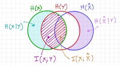
Figure 4: A Venn diagram visualizing $X\rightarrow Y\rightarrow {\hat {X}}$.

We can further recognize that for $E=1$, or equivalently when ${\hat {X}}\neq X$, we know that ${\hat {X}}$ is not equal to the actual value of $X$, thus reducing the possible values of $X$ from $\left|\chi \right|$ to $\left|\chi \right|-1$, thus:

$H\left(X\mid E=1,{\hat {X}}\right)\leq \log _{2}\left(\left|\chi \right|-1\right)$

(40)

This allows us to write Eq. 38 as:

$P_{e}\geq {\frac {H\left(X\mid Y\right)-1}{\log _{2}\left(\left|\chi \right|-1\right)}}$

(41)

And since $H\left(X\mid Y\right)=H\left(X\right)-I\left(X;Y\right)$, we get:

$P_{e}\geq {\frac {H\left(X\right)-I\left(X;Y\right)-1}{\log _{2}\left(\left|\chi \right|-1\right)}}$

(42)

Thus, Fano's inequality leads to a lower bound on the probability of error, for any decoding function ${\hat {X}}=g\left(Y\right)$, and it depends on the mutual information $I\left(X;Y\right)$, or how much information about $X$ is contained in $Y$, and the size of the alphabet $\left|\chi \right|$. Thus, to reduce the lower bound of $P_{e}$, we should minimize $H\left(X\mid Y\right)$, or equivalently maximize $I\left(X;Y\right)$, as expected.

161-A4.1 Activity A4.1 The Data Processing Inequality and Fano's Inequality -- This activity introduces the concept of information loss and the error probabilities associated with entropy and mutual information.

Sources

• Yao Xie's lecture on Data Processing Inequality.