Noise in LTI Systems

Figure 1: Injecting noise in LTI systems.
Once we have our device models with the appropriate noise generators, we can determine the effects of these individual noise sources on the behavior of larger circuits. Consider the linear and time invariant (LTI) system with transfer function  shown in Fig. 1. If we inject noise
  , we would get:
-
 |
|
(1)
|
Thus, the output noise spectrum is shaped or "filtered" by the magnitude of the transfer function. Note that the phase is random and cannot be determined. The total integrated noise at the output of the LTI system is:
-
 |
|
(2)
|
Passive Circuits

Figure 2: Noise in passive circuits.
For the generalized passive circuit shown in Fig. 2, composed of only "noisy" resistors, plus ideal capacitors and inductors, and with an effective impedance across terminals  and
and  equal to
  , the equivalent "spot noise" noise is:
-
![{\displaystyle {\overline {v_{eq}^{2}}}=4kT\cdot \operatorname {Re} \left[Z\left(f\right)\right]\cdot \Delta f}](https://en.wikipedia.org/api/rest_v1/media/math/render/svg/40d1703f409fb1861fdeece62ea0058cd86b20ec) |
|
(3)
|
Note that since is frequency dependent, the spectral density of the noise is shaped by the inductors and capacitors, even though only the resistors generate noise. We can then calculate the total integrated noise:
-
![{\displaystyle {\overline {v_{eq,T}^{2}}}=\int _{B}4kT\cdot \operatorname {Re} \left[Z\left(f\right)\right]\cdot df}](https://en.wikipedia.org/api/rest_v1/media/math/render/svg/cf3c91f5ec5e7aa9d6550b789301c6497d9c3b96) |
|
(4)
|
Example: An RC Circuit
Given the RC circuit in Fig. 3, we can calculate the equivalent impedance seen at the two terminals as:
-
 |
|
(5)
|
Where  . Thus, the total integrated noise is:
-
![{\displaystyle {\begin{aligned}{\overline {v_{eq,T}^{2}}}&=\int _{B}4kT\cdot \operatorname {Re} \left[Z\left(f\right)\right]\cdot df={\frac {4kT}{2\pi }}\int _{0}^{\infty }{\frac {G}{G^{2}+\omega ^{2}C^{2}}}\cdot d\omega \\&={\frac {kT}{C}}\end{aligned}}}](https://en.wikipedia.org/api/rest_v1/media/math/render/svg/674cf6e1487a2ae0d99916a3a69bd2abc265d40e) |
|
(6)
|
Note that the total integrated noise is independent of  . This is due to the fact that the thermal noise spectral density is proportional to , but the bandwidth is inversely proportional to , thus cancelling each other out.
Two-Port Noise Analysis
In general, we perform noise analysis in the small signal domain since, for most circuits, the noise signals are relatively small, allowing us to use superposition. Thus, for a circuit with "noisy" elements, we can calculate the noise seen at any port, e.g. the output port, as:
-
 |
|
(7)
|
Where  is the noise from the
  noise source,
  is the gain from noise source to the port of interest when all other noise sources and inputs are set to zero, and we also assume the noise sources are independent of each other.
Input Equivalent Noise Generators
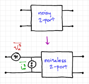
Figure 4: Input equivalent noise generators.
The output noise is a convenient metric to show how "noisy" a circuit is, since it is easy to measure. However, comparing the noise performance of different circuits solely based on the output noise can lead to erroneous results since the output noise also depends on the circuit gain. Hence, we are not sure if a large output noise is due to the inherent noise of the circuit, or possibly due to a relatively large gain. In order to remove this dependency on the circuit gain, we can instead model a "noisy" two-port network using input equivalent noise generators, as shown in Fig. 4.
Thus, we can replace any noisy two-port network with a noiseless two-port network and (1) an equivalent input voltage noise source,  , and (2) an equivalent current noise source,
  . Note that in general, these noise sources are correlated, but let us ignore the correlation for now.
We can calculate by shorting the input, calculating the output noise, then dividing the output noise with the square of the transfer function from the input voltage to the output. Note that by shorting the input, all the current from flows into the short, thus, only contributes to the output noise, as shown in Fig. 5. Similarly, we can calculate by leaving the input open-circuited, calculating the output noise, then dividing the output noise by the square of the transfer function from the input current to the output. Again, when we open-circuit the input, only the input current noise generator contributes to the output noise, as seen in Fig. 6.
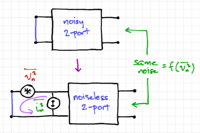 Figure 5: Calculating . |
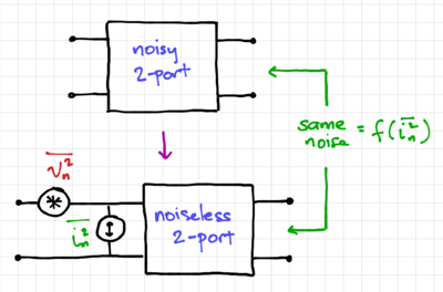 Figure 6: Calculating . |
Example: BJT Input Equivalent Noise
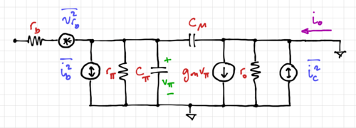
Figure 7: The small signal model of a noisy common-emitter amplifier.
Let us calculate the input equivalent noise of a common-emitter BJT amplifier, whose small signal model is shown in Fig. 7. To get the input equivalent current noise generator, , we open-circuit the base. Note the transfer functions  and
and  . The short-circuit output current noise is then:
-
 |
|
(8)
|
Thus, we get the input equivalent current noise generator:
-
 |
|
(9)
|
To obtain the input equivalent noise generator , we short-circuit the base. Again note that  where
where  . Thus,
-
 |
|
(10)
|
The input equivalent voltage noise generator is then:
-
 |
|
(11)
|
Thus, at low frequencies:
-
 |
|
(12)
|
-
 |
|
(13)
|
The Effect of Source Resistance
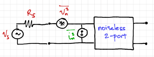
Figure 8: Driving a noisy two-port network with a source resistance

.
Let be the resistance of a source driving a two-port network, shown in Fig. 8. For the extreme case when  , only determines the output noise since the input looks like a short circuit when calculating the output noise. For the other extreme case when
  , the output noise is solely determined by . Thus, we can see that the output noise is dependent on the source resistance . Therefore, intuitively, for large , we want amplifiers with low , e.g. a MOSFET-based amplifier, while for small , we want amplifiers with low , e.g. amplifiers using BJTs.
If the two-port network in Fig. 8 has a voltage gain  and an input impedance
  , we can express the output noise as:
-
 |
|
(14)
|
If we define  , we can calculate the noise figure as:
-
 |
|
(15)
|
If we further define  and
and  as:
as:
-
 |
|
(16)
|
-
 |
|
(17)
|
We get:
-
 |
|
(18)
|
Since appears both at the numerator and denominator, we can conclude that there must be a value of that minimizes the noise figure. Thus, taking the derivative of  with respect to , we get:
-
 |
|
(19)
|
Gives us:
-
 |
|
(20)
|
Note that this assumes that and are uncorrelated. We can then calculate the minimum noise figure:
-
 |
|
(21)
|
Therefore, for a given , there is an optimal ratio of to , or alternatively, for a given amplifier, there is an optimal source resistance that will give us the minimum noise figure. If we take the difference between an amplifier noise figure and the minimum noise figure, we get:
-
 |
|
(22)
|
Or equivalently:
-
 |
|
(23)
|
Where  and
and  . We can then calculate how far our circuit is from the minimum noise figure, given how far we are from the optimal source resistance. Thus, is sometimes called the noise sensitivity parameter. We want to minimize so that the noise match is not too sensitive to the changes in
  .
.
Example: BJT Noise Figure
Recall from the previous example that:
-
 |
|
(24)
|
-
 |
|
(25)
|
Thus, the noise figure for the common-emitter BJT amplifier, driven by a source with source resistance , is:
-
 |
|
(26)
|
Correlated Noise Sources
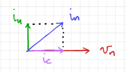
Figure 9: Correlated input equivalent noise sources.
If and are correlated, we can partition the noise current into two components: (1)  , the component uncorrelated to
  , and (2)
  , the component correlated to , such that:
-
 |
|
(27)
|
As shown in Fig. 9. Since and are independent, we can write the dot product as:
-
 |
|
(28)
|
Since and are correlated, we define the admittance  as:
as:
-
 |
|
(29)
|
Thus, the input equivalent voltage noise is:
-
 |
|
(30)
|
Then we can express the noise power at the input as:
-
 |
|
(31)
|
The noise figure is then:
-
 |
|
(32)
|
If we let ,  , and
, and  , we then get:
-
 |
|
(33)
|
And if we further define  and
and  , then to minimize the noise figure, we get:
-
 |
|
(34)
|
-
 |
|
(35)
|
We then get an expression for the minimum noise figure:
-
 |
|
(36)
|
Note that for  , we arrive at the minimum noise figure for the uncorrelated case. And similarly, the noise figure, in terms of
  can be expressed as:
-
 |
|
(37)
|
Where  . Again, if we cannot achieve the optimum source admittance or if we have significant variations in our system, we want to minimize to reduce the sensitivity of the noise figure to the "distance" between the actual source admittance and the optimal source admittance.


