Joint Entropy, Conditional Entropy, and Mutual Information

Joint Entropies

In this module, we'll discuss several extensions of entropy. Let's begin with joint entropy. Suppose we have a random variable $X$ with elements $\{x_{1},x_{2},...,x_{i},...,x_{n}\}$ and random variable $Y$ with elements $\{y_{1},y_{2},...,y_{j},...,y_{m}\}$. We define the joint entropy of $X$ and $Y$ as:

$H(X,Y)=-\sum _{i=1}^{n}\sum _{j=1}^{m}P(x_{i},y_{j})\log _{2}\left(P(x_{i},y_{j})\right)$

Equation 1

Take note that $H(X,Y)=H(Y,X)$. This is trivial. From our previous discussion about the decision trees of a game, we used joint entropies to calculate the overall entropy.

Conditional Entropies

There are two steps to understand conditional entropies. The first is the uncertainty of a random variable caused by a single outcome only. Suppose we have the same random variables $X$ and $Y$ defined earlier in joint entropies. Let's denote $P(y_{j}|x_{i})$ as the conditional probability of $y_{j}$ when event $x_{i}$ happened. We define the entropy $H(Y|x_{i})$ as the entropy of the random variable $Y$ given a $x_{i}$ happened. In other words, this is the average information of all the outcomes of $Y$ when event $x_{i}$ happens. Take note that we're only interested in the entropy of $Y$ when only the outcome $x_{i}$ occurred. Mathematically this is:

$H(Y|x_{i})=-\sum _{j=1}^{m}P(y_{j}|x_{i})\log _{2}\left(P(y_{j}|x_{i})\right)$

Equation 2

Just to repeat because it may be confusing, equation 2 just pertains to the uncertainty when only a single event happened. We can extend this to the total entropy $Y$ when any of the outcomes in $X$ happens. If we treat $H(Y|\cdot )$ like a random variable that contains a range of $\{H(Y|x_{1}),H(Y|x_{2}),H(Y|x_{3}),...,H(Y|x_{n})\}$ and the probability distribution for each associated $H(Y|x_{i})$ is $\{P(x_{1}),P(x_{2}),P(x_{3}),...P(x_{n})\}$ so that $H(Y|\cdot )$ is a function of $X$. Then we define $H(Y|X)$ as the conditional probability of $Y$ given $X$ as:

$H(Y|X)=E(H(Y|\cdot ))=\sum _{i=1}^{n}P(x_{i})H(Y|x_{i})$

Equation 3

Substituting equation 2 to equation 3 and knowing that $P(y_{j}|x_{i})P(x_{i})=P(x_{i},y_{j})$. We can re-write this as:

$H(Y|X)=-\sum _{i=1}^{n}\sum _{j=1}^{m}P(x_{i},y_{j})\log _{2}(P(y_{j}|x_{i}))$

Equation 3 - Better Alternative

Note that it is trivial to prove that $H(Y|X)=H(Y)$ if $Y$ and $X$ are independent. We'll leave it up to you to prove this. A few hints include: $P(y_{j}|x_{i})=P(y_{j})$ and $P(y_{j},x_{i})=P(x_{i})P(y_{j})$ if $Y$ and $X$ are independent.

Binary Tree Example

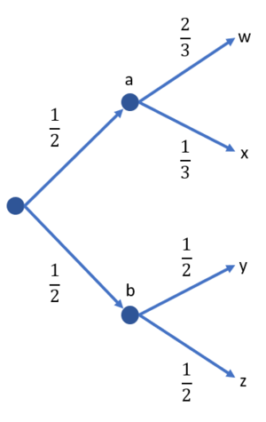
Figure 1: Binary tree example.

Let's apply the first two concepts in a simple binary tree example. Suppose we let $X$ be a random variable with outcomes $\{a,b\}$ and probabilities $\{P(a)=P(b)={\frac {1}{2}}\}$. Let $Y$ be the random variable with outcomes $\{w,x,y,z\}$. We are also given the probabilities $P(w|a)={\frac {2}{3}}$, $P(x|a)={\frac {1}{3}}$, $P(y|b)={\frac {1}{2}}$, and $P(z|b)={\frac {1}{2}}$. Figure 1 shows the binary tree. Calculate:

(a) $H(Y|a)$

(b) $H(Y|b)$

(c) $H(Y|X)$

(d) $H(X,Y)$

Solution

(a) Use equation 2 to solve $H(Y|a)$

${\begin{aligned}H(Y|a)&=-P(w|a)\log _{2}(P(w|a))-P(x|a)\log _{2}(P(x|a))\\&=-{\frac {2}{3}}\log _{2}({\frac {2}{3}})-{\frac {1}{3}}\log _{2}({\frac {1}{3}})\\&=0.918\ {\textrm {bits}}\end{aligned}}$

(b) Same as in (a), use equation 2 to solve $H(Y|b)$

${\begin{aligned}H(Y|b)&=-P(y|b)\log _{2}(P(y|b))-P(z|b)\log _{2}(P(z|b))\\&=-{\frac {1}{2}}\log _{2}({\frac {1}{2}})-{\frac {1}{2}}\log _{2}({\frac {1}{2}})\\&=1.000\ {\textrm {bits}}\end{aligned}}$

(c) Can be solved in two ways. First is to use equation 3.

${\begin{aligned}H(Y|X)&=E(H(Y|\cdot ))\\&=P(a)H(Y|a)+P(b)H(Y|b)\\&={\frac {1}{2}}(0.918)+{\frac {1}{2}}(1.000)\\&=0.959\ {\textrm {bits}}\end{aligned}}$

Or, we can solve it using the alternative version of equation 3. But we also need to know the joint probabilities:

• $P(a,w)={\frac {1}{3}}$
• $P(a,x)={\frac {1}{6}}$
• $P(b,y)={\frac {1}{4}}$
• $P(b,z)={\frac {1}{4}}$

${\begin{aligned}H(Y|X)&=-\sum _{i=1}^{n}\sum _{j=1}^{m}P(x_{i},y_{j})\log _{2}(P(y_{j}|x_{i}))\\&=-P(w,a)\log _{2}(P(w|a))-P(x,a)\log _{2}(P(x|a))-P(y,b)\log _{2}(P(y|b))-P(z,b)\log _{2}(P(z|b))\\&=-{\frac {1}{3}}\log _{2}\left({\frac {2}{3}}\right)-{\frac {1}{6}}\log _{2}\left({\frac {1}{3}}\right)-{\frac {1}{4}}\log _{2}\left({\frac {1}{2}}\right)-{\frac {1}{4}}\log _{2}\left({\frac {1}{2}}\right)\\&=0.959\ {\textrm {bits}}\end{aligned}}$

(d) We already listed the joint probabilities in (c). We simply use equation 1 for this:

${\begin{aligned}H(X,Y)&=-\sum _{i=1}^{n}\sum _{j=1}^{m}P(x_{i},y_{j})\log _{2}\left(P(x_{i},y_{j})\right)\\&=-P(a,w)\log _{2}(P(a,w))-P(a,x)\log _{2}(P(a,x))-P(b,y)\log _{2}(P(b,y))-P(b,z)\log _{2}(P(b,z))\\&=-{\frac {1}{3}}\log _{2}\left({\frac {1}{3}}\right)-{\frac {1}{6}}\log _{2}\left({\frac {1}{6}}\right)-{\frac {1}{4}}\log _{2}\left({\frac {1}{4}}\right)-{\frac {1}{4}}\log _{2}\left({\frac {1}{4}}\right)\\&=1.959\ {\textrm {bits}}\end{aligned}}$

Important Note!

This example actually shows us an important observation:

$H(X,Y)=H(X)+H(Y|X)$

Equation 4

We can easily observe that this holds true for the binary tree example. This has an important interpretation: The combined uncertainty in $X$ and $Y$ (i.e., $H(X,Y)$) is the sum of that uncertainty which is totally due to $X$ (i.e., $H(X)$), and that which is still due to $Y$ once $X$ has been accounted for (i.e., $H(Y|X)$).

Since $H(X,Y)=H(Y,X)$ it also follows that:

$H(Y,X)=H(Y)+H(X|Y)$

Equation 5

If $X$ and $Y$ are independent then:

$H(X,Y)=H(X)+H(Y)$

Equation 6

An alternative interpretation to $H(Y|X)$ is the information content of $Y$ which is NOT contained in $X$.

Mutual Information

With the final discussion on the properties of joint and conditional entropies, we also define mutual information as the information content of $Y$ contained within $X$ written as:

$I(X,Y)=H(Y)-H(Y|X)$

Equation 7

Or:

$I(X,Y)=H(X)-H(X|Y)$

Equation 7 - Alternative

If we plug in the definitions of entropy and conditional entropy, mutual information in expanded form is:

$I(X,Y)=\sum _{i=1}^{n}\sum _{j=1}^{m}P(x_{i},y_{j})\log _{2}\left({\frac {P(x_{i},y_{j})}{P(x_{i})P(y_{j})}}\right)$

Equation 8

It also follows that:

• $I(X,Y)=I(Y,X)$. This is trivial from equation 7.
• If $X$ and $Y$ are independent, then $I(X,Y)=0$. This is also trivial from equation 8.

As a short example, we can use the binary tree problem again. Let's compute $I(X,Y)$. We simply need to use equation 7: $I(X,Y)=H(Y)-H(Y|X)$. We already know $H(Y|X)=0.959$ bits. $H(Y)$ is computed by first knowing $\{P(w),P(x),P(y),P(z)\}$. Recall that:

$P(y_{j})=\sum _{i=1}^{n}P(y_{j}|x_{i})P(x_{i})$

But then, for each outcome in $Y$ has the same probability of the joint entropy. For example, event $w$ only occurs if event $a$ occurred first. Event $y$ occurs only if event $b$ occurred first. So it means that:

• $P(w)=P(w|a)P(a)=P(w,a)={\frac {1}{3}}$
• $P(x)=P(x|a)P(a)=P(x,a)={\frac {1}{6}}$
• $P(y)=P(y|b)P(b)=P(y,b)={\frac {1}{4}}$
• $P(z)=P(z|b)P(b)=P(z,b)={\frac {1}{4}}$

Therefore, $H(Y)=H(X,Y)=1.959$ bits. Therefore, the information $I(X,Y)=H(Y)-H(Y|X)=1.959-0.959=1.000$ bits.

Chain Rule for Conditional Entropy

What happens when we deal with more than two random variables? To facilitate the discussion, let us recall the chain rule for joint distributions.

Let $X_{1},X_{2},...,X_{n}$ be a sequence of discrete random variables. Then, their joint distribution can be factored as follows

$p(X_{1},X_{2},...X_{n})=p(X_{1})p(X_{2}|X_{1})p(X_{3}|X_{1},X_{2})...p(X_{n}|X_{1},X_{2},...X_{n-1})$,

Chain rule for entropy

The chain rule for (joint) entropy is very similar to the above expansion, but we use additions instead of multiplications.

$H(X_{1},X_{2},...,X_{n})=H(X_{1})+H(X_{2}|X_{1})+H(X_{3}|X_{1},X_{2})+...+H(X_{n}|X_{1},X_{2},...,X_{n-1})$

Equation 9

Although we do not supply a complete proof here, this fact should not be too surprising since entropy operates on logarithms of probabilities and logarithms of product terms expand to sums of logarithms.

Proof of chain rule for $n=3$

Let us see that the statement is true for $n=3$. Let $X_{1},X_{2},X_{3}$ be three discrete random variables. The idea with the proof is that we operate on two random variables at a time, since prior to the chain rule we only know that $H(X,Y)=H(X)+X(Y|X)$. We can write $H(X_{1},X_{2},X_{3})=H((X_{1},X_{2}),X_{3})$, where we bundle $X_{1}$ and $X_{2}$ into one random variable $(X_{1},X_{2})$.

The proof now proceeds as follows:

$H(X_{1},X_{2},X_{3})=H((X_{1},X_{2}),X_{3})=H(X_{1},X_{2})+H(X_{3}|X_{1},X_{2})=[H(X_{1})+H(X_{2}|X_{1})]+H(X_{3}|X_{1},X_{2})$

One interpretation of the chain rule shown is that to obtain the total information (joint entropy) of $X_{1},X_{2},X_{3}$ as a whole, we can

• obtain information about $X_{1}$ first without any prior knowledge: $H(X_{1})$, then
• obtain information about $X_{2}$ with knowledge of $X_{1}$: $H(X_{2}|X_{1})$, then
• obtain information about $X_{3}$ with knowledge of $X_{1}$ and $X_{2}$: $H(X_{3}|X_{1},X_{2})$.

For $n>3$, we can proceed by induction. Below is the sketch of the proof:

• (Base step) For a fixed $n=k$, assume that any collection of $k$ random variables satisfies the chain rule.
• (Induction step) When $n=k+1$, write the joint entropy of $k+1$ random variables as follows: $H(X_{1},...,X_{k},X_{k+1})=H((X_{1},...,X_{k}),X_{k+1})$, where the first $k$ are bundled together into one random variable.
• Use the two-variable chain rule $H(X,Y)=H(X)+H(Y|X)$ and the base step to show that $H(X_{1},...,X_{k},X_{k+1})=H(X_{1})+H(X_{2}|X_{1})+...+H(X_{k+1}|X_{1},...,X_{k})$.

A few things to note:

• The order of "obtaining information" is irrelevant in calculating the joint entropy of multiple rvs. Write the chain rule if we proceed by obtaining information in the following order: $X_{2},X_{3},X_{1}$.
• The chain we have now works for any collection of random variables. Can you figure out how to simplify the chain rule for Markov chains? (The answer will be discussed in Module 3.)

Graphical Summary

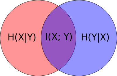
Figure 2 shows how we can visualize conditional entropy and mutual information. The red and blue pertain to the individual entropies $H(X)$ and $H(Y)$, respectively. Figure 3 shows what joint entropy looks like.

Figure 2: Venn diagram visualizing conditional entropy and mutual information.

Figure 3: Venn diagram visualizing joint entropy.

From the diagrams you should be able to recall the entropy relationships on the fly. We can summarize (and derive new relationships) as:

• $I(X,Y)=H(X)-H(X|Y)=H(Y)-H(Y|X)$
• $H(X,Y)=H(X|Y)+H(Y|X)+I(X,Y)=H(X)+H(Y)-I(X,Y)$

From the diagrams, it's easy to re-translate $H(Y|X)$ (or $H(X|Y)$) as the uncertainty of $Y$ without the $X$ happening

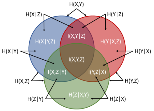
Of course we, can extend this concept to three variables. For example, figure 4 shows a Venn diagram for three sets. The entire blue circle is $H(X)$, the entire red is $H(Y)$, and the entire green is $H(Z)$. The labels are there to guide you.

Figure 4: Entropy Venn diagram from three sets.

We can also derive useful relationships based on figure 4. Some of these include:

• $H(X,Y,Z)=H(X)+H(Y|X)+H(Z|X,Y)$ which is consistent with equation 9. Look at the diagram carefully.
• $H(X,Y,Z)=H(X)+H(Y)+H(Z)-I(X,Y)-I(Y,Z)-I(X,Z)+I(X,Y,Z)$ while noting that $I(X,Y)=H(X,Y)-H(X|Y)-H(Y|X)$, $I(X,Z)=H(X,Z)-H(X|Z)-H(Z|X)$, and $I(Y,Z)=H(Y,Z)-H(Z|Y)-H(Y|Z)$.
• $I(X,Y,Z)=H(X,Y,Z)-H(X)-H(Y)-H(Z)+I(X,Y)+I(Y,Z)+I(X,Z)$ as a consequence of the previous equation.
• $I(X,Y|Z)=H(X,Y,Z)-H(Z)-H(X|Y,Z)-H(Y|X,Z)$. All similar combinations (e.g., $I(X,Z|Y)$ and $I(Y,Z|X)$ ) should be the same too.