The Ideal Integrator
The ideal integrator, shown in Fig. 1, with symbol shown in Fig. 2, makes use of an ideal operational amplifier with  ,
,  , and
, and  .
.
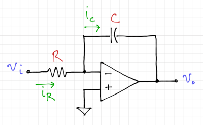 Figure 1: The op-amp-based ideal integrator. |
 Figure 2: The symbol for an integrator. |
The current through the resistor,  , can be expressed as:
-
 |
|
(1)
|
Thus, we can write the integrator output voltage,  , as:
, as:
-
 |
|
(2)
|
In the Laplace domain:
-
 |
|
(3)
|
Or equivalently:
-
 |
|
(4)
|
The magnitude and phase response of an ideal integrator is shown in Figs. 3 and 4. A key feature to note in ideal integrators is the fact that:
- The unity gain frequency is equal to
 , and
, and
- The phase at the unity gain frequency is exactly
 .
.
 Figure 3: Magnitude response of an ideal integrator with  . |
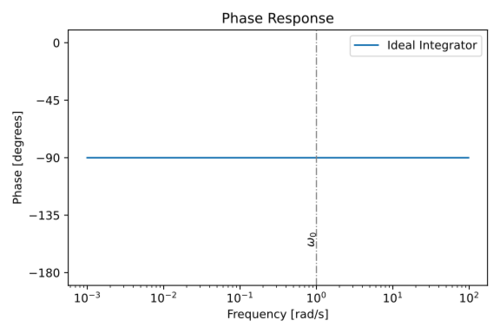 Figure 4: Phase response of an ideal integrator with . |
Rewriting the transfer function as:
-
 |
|
(5)
|
We can then define the quality factor of an ideal integrator:
-
 |
|
(6)
|
Since  . Fig. 5 shows a two-input integrator, with output voltage:
-
 |
|
(7)
|
 Figure 5: A two-input op-amp integrator. |
Integrator Noise
Fig. 6 shows an integrator where the output is fed back to one of its inputs, giving us:
-
 |
|
(8)
|
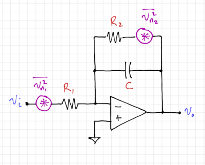 Figure 6: Resistor thermal noise generators in an integrator. |
Ignoring the noise from the amplifier, the output noise of the integrator in Fig. 6 can be expressed as:
-
 |
|
(9)
|
The total integrated noise is then:
-
 |
|
(10)
|
Integrator Non-Idealities
In practice, integrators are limited by the characteristics of non-ideal amplifiers: (1) finite gain at DC, and (2) non-dominant amplifier poles. Let us look at the effects of these non-idealities one at a time.
Finite Gain
The transfer function of an integrator using an amplifier with finite gain,  , can be written as:
-
 |
|
(11)
|
The magnitude and phase response of this non-ideal integrator is shown in Figs. 7 and 8.
 Figure 7: The magnitude response of an integrator with a finite-gain amplifier. |
 Figure 8: The phase response of an integrator with a finite-gain amplifier. |
Note that the integrator quality factor now becomes finite:
-
 |
|
(12)
|
The phase at  is then:
-
 |
|
(13)
|
Thus, if is finite,  will approach, but will never be equal to , resulting in a phase lead. For example, if
  , we get
  , and
, and  will result in
  .
.
Non-Dominant Poles
The transfer function of an integrator using an amplifier with infinite gain but with non-dominant poles can be expressed as:
-
 |
|
(14)
|
The magnitude and phase response of this non-ideal integrator is shown in Figs. 9 and 10.
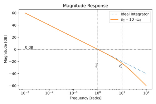 Figure 9: The magnitude response of an integrating using an amplifier with a non-dominant pole,  . |
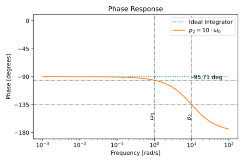 Figure 10: The phase response of an integrating using an amplifier with a non-dominant pole, . |
The phase at the unity gain frequency is then equal to:
-
 |
|
(15)
|
Note that the non-dominant poles contribute to the integrator phase lag.
In a real integrator, the effects (phase lead) of the amplifier finite gain can cancel out the effects (phase lag) of the non-dominant poles! Given the transfer function of the integrator with an amplifier that has both finite gain and non-dominant poles:
-
 |
|
(16)
|
If we assume that  and
and  , we can then rewrite the transfer function as:
-
 |
|
(17)
|
For  non-dominant poles. The integrator quality factor is then equal to:
-
 |
|
(18)
|
As expected, the effect of finite gain can be cancelled out by the effect of the non-dominant poles.
Capacitor Non-Idealities
For lossy capacitors, modeled in Fig. 11 as an ideal capacitor in series with a resistor,  , the integrator transfer function becomes:
-
 |
|
(19)
|
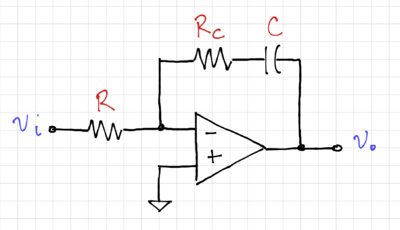 Figure 11: An integrator with a lossy capacitor. |
The magnitude and phase response is shown in Figs. 12 and 13.
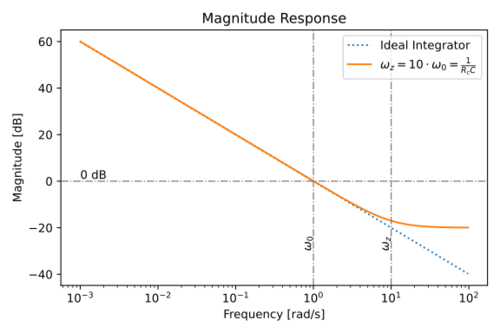 Figure 12: Magnitude response of an integrator with a lossy capacitor. |
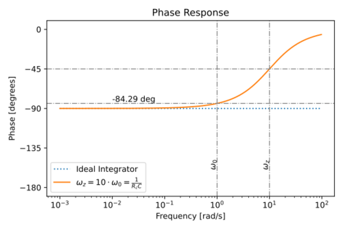 Figure 13: Magnitude response of an integrator with a lossy capacitor. |
Notice the phase lead introduced by the zero due to . At :
-
 |
|
(20)
|
The integrator quality factor can then be written as:
-
 |
|
(21)
|
Thus, a non-zero degrades the integrator quality factor, but in typical implementations, the amplifier non-idealities will dominate.
 Integrators
An alternative implementation of an integrator is to use transconductances, which drive constant current into capacitors, as shown in Fig. 14.
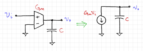 Figure 14: A integrator. |
We can write the output voltage as:
-
 |
|
(22)
|
Where  . This type of integrator is ideal in cases where the loads are capacitive, e.g. in CMOS circuits, and are much simpler than op-amp-based integrators since integrators are open-loop circuits without feedback. In general, real transconductance amplifiers will have transconductances that vary with frequency,
  , thus also affecting the phase at , similar to op-amp-based integrators.
Summary
The quality factor of the integrator is reduced by:
- The finite gain of the amplifier,
- The presence of amplifier non-dominant poles, and
- The loss of passive reactive components, e.g. capacitors.
Note that both the finite amplifier gain and the lossy capacitor introduces a phase lead, and the presence of non-dominant poles results in a phase lag.


