Filter Synthesis

Filters can be implemented (1) as a cascade if biquadratic filters, or biquads, that implements one or two poles at a time, or (2) as ladder filters.

Biquadratic Filters

To implement a single real pole, we can use a simple RC cicuit, as shown in Fig. 1, whose transfer function is given by:

$H\left(s\right)={\frac {1}{1+sRC}}$

(1)

To implement two complex conjugate poles, we can use a lossy LC circuit, as shown in Fig. 2. We can then express the transfer function of this circuit as:

$H\left(s\right)={\frac {1}{s^{2}LC+s{\frac {L}{R}}+1}}$

(2)

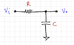Figure 1: A simple RC circuit.

Figure 2: A lossy RLC circuit.

A more complex filter can then be implemented by cascading 2-pole filters, and an extra 1-pole filter for odd-order complex filters, as shown in Fig. 3 for a fifth order filter. Note that (1) filters built as a cascade of biquads are easy to implement, but they are very sensitive to mismatch since the filter transfer function is dependent not only on the pole locations, but on the pole placement relative to other poles, (2) buffers are used to prevent loading effects, and (3) the biquads are arranged from lowest to highest Q to help reduce loss and noise.

Figure 3: A 5th order filter implemented using cascaded biquads.

Ladder Networks

A better alternative to cascading biquads is to expand the filter's driving point or input impedance using continued fraction expansion. Consider a general ladder network shown in Fig. 4. The input impedance, $Z_{11}$, can then be expressed as the continued fraction:

$Z_{11}={\cfrac {1}{Y_{1}+{\cfrac {1}{Z_{2}+{\cfrac {1}{Y_{3}+\ldots +{\cfrac {1}{Z_{N-1}+{\cfrac {1}{Y_{N}}}}}}}}}}}$

(3)

Thus, we can build filters using ladder networks if we know their input impedance.

Figure 4: A general ladder network.

Example: A Low-Pass Butterworth Filter

Consider a third order low-pass Butterworth filter with the normalized (to $\omega _{0}=1\,\mathrm {\tfrac {rad}{s}}$) transfer function:

$H\left(s\right)={\frac {N\left(s\right)}{D\left(s\right)}}={\frac {1}{s^{3}+2s^{2}+2s+1}}$

(4)

The filter is shown in Fig. 5, where it is driven by a source with input resistance, $R_{S}$, and loaded by the resistance, $R_{L}$.

Figure 5: A filter driven by a source with resistance, $R_{S}$, and driving a resistive load, $R_{L}$.

For the normalized impedance case, where $R_{S}=R_{L}=1\,\mathrm {\Omega }$, and with $N=3$:

${\begin{aligned}Z_{11}&={\frac {D\left(s\right)-s^{N}}{D\left(s\right)+s^{N}}}\\&={\frac {s^{3}+2s^{2}+2s+1-s^{3}}{s^{3}+2s^{2}+2s+1+s^{3}}}\\&={\frac {2s^{2}+2s+1}{2s^{3}+2s^{2}+2s+1}}\end{aligned}}$

(5)

We can then expand this as:

${\begin{aligned}Z_{11}&={\cfrac {1}{\cfrac {s^{3}+2s^{2}+2s+1+s^{3}}{2s^{2}+2s+1}}}\\&={\cfrac {1}{s+{\cfrac {s+1}{2s^{2}+2s+1}}}}\\&={\cfrac {1}{s+{\cfrac {1}{\frac {2s^{2}+2s+1}{s+1}}}}}\\&={\cfrac {1}{s+{\cfrac {1}{2s+{\cfrac {1}{s+1}}}}}}\\\end{aligned}}$

(6)

Thus, for the low-pass case, we have capacitors as the admittances to ground, and inductors as the impedances in the forward path, or equivalently $Y_{i}=sC_{i}$ and $Z_{i}=sL_{i}$, and in the terminated case, $Y_{N}=sC_{N}+{\tfrac {1}{R_{L}}}$. We can then determine the capacitance and inductance values of the third order low-pass Butterworth filter:

${\begin{aligned}Y_{1}=s&\rightarrow C_{1}=1\,\mathrm {F} \\Z_{2}=s&\rightarrow L_{2}=2\,\mathrm {H} \\Y_{3}=s&\rightarrow C_{3}=1\,\mathrm {F} \\\end{aligned}}$

(7)

The resulting filter is shown in Fig. 6.

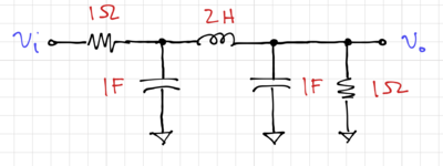Figure 6: A third order low-pass normalized Butterworth filter.

Filter Tables

For higher-order filters, calculating the inductance and capacitance values could take some time and effort, though these values are well known. An alternative to continued fraction expansion, in implementing ladder filters, is the use of filter tables. Fig. 8 shows a sample filter table taken from the famous book by Anatoly Zverev. To illustrate the use of filter tables, consider the example below.

Filter Design Example

Let us design a filter with the following specifications:

• A maximally flat low-pass filter
• A cut-off frequency, $f_{0}=10\,\mathrm {MHz}$
• An attenuation of at least $27\,\mathrm {dB}$ at $f_{\text{stop}}=20\,\mathrm {MHz}$

Step 1: Determine the filter family

Let us use the Butterworth low-pass filter prototype since it has a maximally flat pass band.

Step 2: Determine the filter order

We can determine the order from the magnitude response of the filter, which we can get using tools like Python or Matlab, or in this case, we can use filter tables and graphs. Fig. 7 shows the Butterworth attenuation characteristics for different filter orders. Note that this graph is normalized to $\omega _{0}=1\,\mathrm {\tfrac {rad}{s}}$.

Figure 7: Attenuation characteristics of Butterworth filters.

To get the lowest order filter that satisfies our requirements, we can then look at the point where:

${\frac {f_{\text{stop}}}{f_{0}}}=2$

(8)

Thus, we can see that we need at least a fifth order filter, i.e. $N=5$.

Step 3: Determine the normalized LC values

We can obtain the inductor and capacitor values of the 5th order low-pass Butterworth filter normalized to $\omega _{0}=1\,\mathrm {\tfrac {rad}{s}}$ from the filter transfer function using continued fraction expansion, or just use a filter table, as shown in Fig. 8.

Figure 8: Butterworth LC element values.

Looking at the entry for $N=5$, with $R_{S}=R_{L}=1\,\mathrm {\Omega }$, we get the normalized values $C_{1,{\text{norm}}}=0.6180\,\mathrm {F}$, $L_{2,{\text{norm}}}=1.6180\,\mathrm {H}$, $C_{3,{\text{norm}}}=2.0000\,\mathrm {F}$, $L_{4,{\text{norm}}}=1.6180\,\mathrm {H}$, and $C_{5,{\text{norm}}}=0.6180\,\mathrm {F}$.

Step 4: Denormalize

Denormalization is the process of shifting the corner frequency from $\omega _{0}=1\,\mathrm {\tfrac {rad}{s}}$ to $\omega _{0}=2\pi \cdot \left(10\,\mathrm {MHz} \right)\,\mathrm {\tfrac {rad}{s}}$. For now, let us leave $R_{S}=R_{L}=R=1\,\mathrm {\Omega }$. We then define $L_{r}={\tfrac {R}{\omega _{0}}}$ and $C_{r}={\tfrac {1}{\omega _{0}R}}$, where $\omega _{0}=2\pi \cdot \left(10\,\mathrm {MHz} \right)\,\mathrm {\tfrac {rad}{s}}$. Thus, in this case, we get:

${\begin{aligned}L_{r}&={\tfrac {R}{\omega _{0}}}={\frac {1\,\mathrm {\Omega } }{2\pi \cdot \left(10\,\mathrm {MHz} \right)}}=15.9\,\mathrm {nH} \\C_{r}&={\tfrac {1}{\omega _{0}R}}={\frac {1}{2\pi \cdot \left(10\,\mathrm {MHz} \right)\cdot \left(1\,\mathrm {\Omega } \right)}}=15.9\,\mathrm {nF} \\\end{aligned}}$

(9)

We can then determine the denormalized element values using $L_{i}=L_{i,{\text{norm}}}\cdot L_{r}$ and $C_{i}=C_{i,{\text{norm}}}\cdot C_{r}$, thus:

${\begin{aligned}C_{1}&=C_{1,{\text{norm}}}\cdot C_{r}=9.836\,\mathrm {nF} \\L_{2}&=L_{2,{\text{norm}}}\cdot L_{r}=25.75\,\mathrm {nH} \\C_{3}&=C_{3,{\text{norm}}}\cdot C_{r}=31.83\,\mathrm {nF} \\L_{4}&=L_{4,{\text{norm}}}\cdot L_{r}=25.75\,\mathrm {nH} \\C_{5}&=C_{5,{\text{norm}}}\cdot C_{r}=9.836\,\mathrm {nF} \\\end{aligned}}$

(10)

The resulting fifth order low-pass Butterworth filter is shown in Fig. 9.

Figure 9: The resulting 5th order low-pass Butterworth filter with $f_{0}=10\,\mathrm {MHz}$.

We can verify the magnitude response of the filter using SPICE, as shown in Fig. 10. Note that the low frequency gain is maximally flat, and is at $-6\,\mathrm {dB}$ due to the voltage division between the source and load resistances.

Figure 10: Fifth order Butterworth filter SPICE simulation result.