Filtering is the oldest and most common type of signal processing, usually in the form of frequency selectivity or phase shaping, or both. Some filter applications include (1) extracting a desired signal from other signals, (2) separating signals from noise, (3) anti-aliasing in analog-to-digital converters or smoothing in digital-to-analog converters, (4) phase equalization, and (5) limiting amplifier bandwidths for reducing noise.
Filter Types
As shown in Figs. 1-5, we can classify filters based on frequency range selectivity as: (1) low-pass filters, (2) high-pass filters, (3) band-pass filters, (4) band-stop, band-reject, or notch filters, and (5) all-pass filters used for phase shaping or equalization.
 Figure 1: Low-pass filter magnitude response and symbol. |
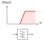 Figure 2: High-pass filter magnitude response and symbol. |
 Figure 3: Band-pass filter magnitude response and symbol. |
 Figure 4: Band-stop filter magnitude response and symbol. |
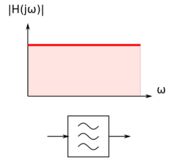 Figure 5: All-pass filter magnitude response and symbol. |
Note that we can easily derive high-pass and band-pass filters from their low-pass equivalents, and thus, even though most of our examples feature low-pass filters, the concepts and ideas are applicable to the other filter types.
Ideal vs. Practical Filters
Let us consider an ideal low-pass filter, whose magnitude response is shown in Fig. 6. This ideal filter response has three properties: (1) it has a flat magnitude in the pass-band, resulting in no amplitude distortion in the signals we are passing, (2) it has a "brick wall" transition region, i.e. the transition between the pass-band and stop-band is abrupt, and (3) it has infinite rejection of out-of-band signals, i.e. zero magnitude response. These characteristics make building an ideal filter rather impractical.
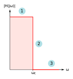 Figure 6: The ideal low-pass filter magnitude response. |
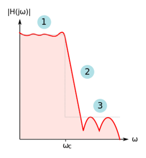 Figure 7: A practical low-pass filter magnitude response. |
A real filter has the following magnitude response properties, as shown in Fig. 7:
- The pass-band could contain ripples, thus causing amplitude distortion in the signals being passed by the filter.
- There is a finite transition region between the pass-band and the stop-band.
- The rejection of stop-band (or out-of-band) signals is finite.
Magnitude and Frequency Metrics
In the design of filters, we can specify the filter specifications using following parameters, as illustrated in Fig. 8:
- DC Pass-band Gain,

- The value of the magnitude transfer function at DC or as
 .
.
- Corner Frequency,

- The corner frequency specification.
- Stop-band Frequency,

- The stop-band frequency specification.
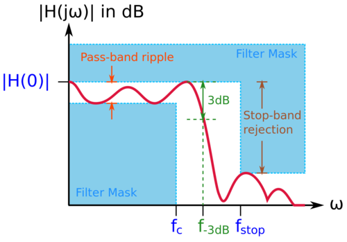 Figure 8: Filter design specifications. |
The frequency range from to is the transition region separating the pass-band from the stop-band. Instead of individual separate metrics, another way of detailing the filter specifications is by using filter mask, also shown in Fig. 8. The filter mask is a graphical representation of the allowable values the filter magnitude response can take.
Group Delay
Aside from the filter magnitude specifications, the filter phase response is also a critical parameter, and we would like to determine the how the phase affects the overall behavior of the filter. Consider a filter with transfer function  , as shown in Fig. 9.
 Figure 9: A 2-port representation of a filter. |
Let us apply two sinusoids:
-
![{\displaystyle v_{i}\left(t\right)=A_{1}\sin \left(\omega t\right)+A_{2}\sin \left[\left(\omega +\Delta \omega \right)t\right]}](https://en.wikipedia.org/api/rest_v1/media/math/render/svg/950d3f7010722bb12c00d7d56dc3422b0bb076ec) |
|
(1)
|
The output can then be written as:
-
![{\displaystyle {\begin{aligned}v_{o}\left(t\right)&=A_{1}\cdot \left|G\left(j\omega \right)\right|\cdot \sin \left[\omega t+\theta \left(\omega \right)\right]+A_{2}\cdot \left|G\left(j\omega +j\Delta \omega \right)\right|\cdot \sin \left[\left(\omega +\Delta \omega \right)t+\theta \left(\omega +\Delta \omega \right)\right]\\&=A_{1}\cdot \left|G\left(j\omega \right)\right|\cdot \sin \left[\omega \left(t+{\frac {\theta \left(\omega \right)}{\omega }}\right)\right]+A_{2}\cdot \left|G\left(j\omega +j\Delta \omega \right)\right|\cdot \sin \left[\left(\omega +\Delta \omega \right)\left(t+{\frac {\theta \left(\omega +\Delta \omega \right)}{\omega +\Delta \omega }}\right)\right]\end{aligned}}}](https://en.wikipedia.org/api/rest_v1/media/math/render/svg/5d41fdc441a6be067e7bf72f20cd49b68ddc5a5e) |
|
(2)
|
Note that the sinusoid at  is delayed differently from the sinusoid at
  , resulting in phase distortion.
Recall that  , thus we can write:
-
 |
|
(3)
|
And also:
-
 |
|
(4)
|
Thus:
-
![{\displaystyle {\begin{aligned}{\frac {\theta \left(\omega +\Delta \omega \right)}{\omega +\Delta \omega }}&\approx \left[\theta \left(\omega \right)+{\frac {\partial \theta \left(\omega \right)}{\partial \omega }}\cdot \Delta \omega \right]\cdot \left[{\frac {1}{\omega }}\left(1-{\frac {\Delta \omega }{\omega }}\right)\right]\\&\approx {\frac {\theta \left(\omega \right)}{\omega }}+{\frac {\partial \theta \left(\omega \right)}{\partial \omega }}\cdot {\frac {\Delta \omega }{\omega }}-{\frac {\theta \left(\omega \right)}{\omega }}\cdot {\frac {\Delta \omega }{\omega }}\\&\approx {\frac {\theta \left(\omega \right)}{\omega }}+\left({\frac {\partial \theta \left(\omega \right)}{\partial \omega }}-{\frac {\theta \left(\omega \right)}{\omega }}\right)\cdot {\frac {\Delta \omega }{\omega }}\end{aligned}}}](https://en.wikipedia.org/api/rest_v1/media/math/render/svg/f3aeb303375056997060256f09a56c5ffbe22545) |
|
(5)
|
We can then write the output as:
-
![{\displaystyle {\begin{aligned}v_{o}\left(t\right)&=A_{1}\cdot \left|G\left(j\omega \right)\right|\cdot \sin \left[\omega \left(t+{\frac {\theta \left(\omega \right)}{\omega }}\right)\right]+A_{2}\cdot \left|G\left(j\omega +j\Delta \omega \right)\right|\cdot \sin \left[\left(\omega +\Delta \omega \right)\left(t+{\frac {\theta \left(\omega +\Delta \omega \right)}{\omega +\Delta \omega }}\right)\right]\\&=A_{1}\cdot \left|G\left(j\omega \right)\right|\cdot \sin \left[\omega \left(t+{\frac {\theta \left(\omega \right)}{\omega }}\right)\right]+A_{2}\cdot \left|G\left(j\omega +j\Delta \omega \right)\right|\cdot \sin \left[\left(\omega +\Delta \omega \right)\left(t+{\frac {\theta \left(\omega \right)}{\omega }}+\delta \right)\right]\end{aligned}}}](https://en.wikipedia.org/api/rest_v1/media/math/render/svg/cee1c9d359440f1c3c1482b7bd03d52b4f8925c6) |
|
(6)
|
Where:
-
 |
|
(7)
|
Let us define phase delay,  as:
as:
-
 |
|
(8)
|
Note that if  , both sinusoids will be delayed in time by , preserving the relative delays of the input sinusoids. If
  , the output at will be time shifted differently than the output at , leading to phase distortion.
To avoid phase distortion, we need to set , or equivalently:
-
 |
|
(9)
|
Thus, solving the differential equation above, we get  , where
  is a constant.
Let us further define group delay,  as:
as:
-
 |
|
(10)
|
Filters with , or equivalently,  , are called linear phase filters, and these filters do not introduce phase distortion. Note that filters with
  , where
  is a constant, are also linear phase filters but are NOT free of phase distortion. Further note that if
  , then we can say that there is no signal magnitude distortion. In most cases, these ideal conditions of no phase or magnitude distortion are not exactly realizable.


