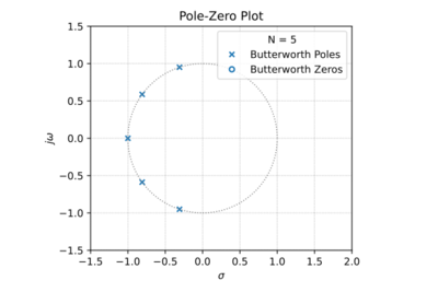
Figure 1: The Butterworth low-pass pole-zero plot for

.
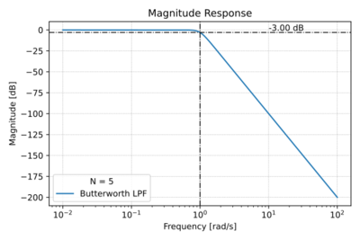
Figure 2: The Butterworth low-pass filter magnitude response for
.
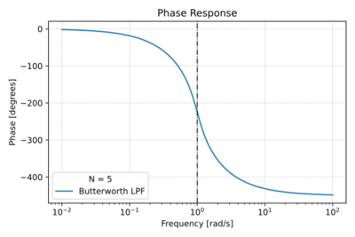
Figure 3: The Butterworth low-pass filter phase response for
.
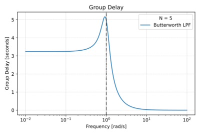
Figure 4: The Butterworth low-pass filter group delay for
.
Butterworth filters are a class of all-pole filters, where the poles of the normalized transfer function are equally spaced along the unit circle ( ), seen in Fig. 1 for . This results in a maximally flat pass-band magnitude response as shown in Fig. 2, or equivalently:
-
 |
|
(1)
|
This means that the  derivative of the magnitude at DC is zero. Note the
  roll-off for , as expected.
The Low-Pass Butterworth Filter
The low-pass Butterworth filter has the following magnitude response:
-
 |
|
(2)
|
Where  is the filter order and
  is the
  frequency. Note that
  at
at  . Thus:
-
 |
|
(3)
|
Thus, the poles are the roots of:
-
 |
|
(4)
|
Or equivalently:
-
 |
|
(5)
|
Since we can write  , the roots of
  can be written as:
-
 |
|
(6)
|
For  . Thus, we get:
-
 |
|
(7)
|
Solving for  , we get the poles of the low-pass Butterworth filter:
-
 |
|
(8)
|
We can then write:
-
 |
|
(9)
|
We can also plot the phase response as illustrated in Fig. 3, and taking the derivative of the phase, we get the group delay plot in Fig. 4. Note that there is moderate phase distortion around .


