229-A2.1

Activity: Nonlinearity in Circuits

• Instructions: This activity is structured as a tutorial with a design problem at the end. Should you have any questions, clarifications, or issues, please contact your instructor as soon as possible.
• At the end of this activity, the student should be able to:

1. Understand and observe the effects of nonlinearity in electronic circuits.

Visualizing Nonlinearity

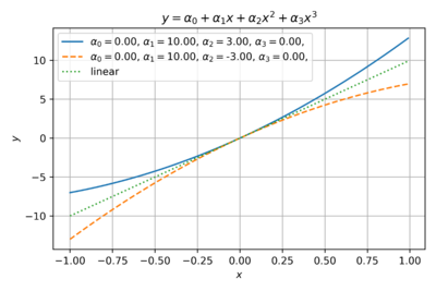
Let us examine the effects of varying the coefficients of the power series model of our transfer function using this Python script. Fig. 1 shows the an even function with only second order coefficients. This is typical of ideal square-law single-ended MOS amplifiers where a quadratic term dominates.

Figure 1: An even function with positive and negative second order coefficients.

Figure 2: An odd function with positive and negative third order coefficients.

Figure 3: A differential amplifier.

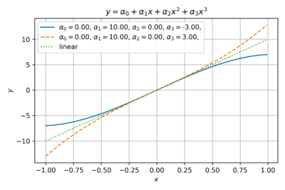
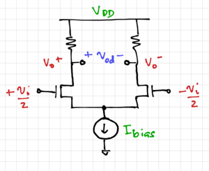
Fig. 2 shows an odd function with only third order coefficients. This is a good estimate for differential circuits, where the common-mode terms cancel out. For example, the outputs of a differential amplifier in Fig. 3 can be expressed as:

$v_{\mathrm {o} }^{+}=\alpha _{0}+\alpha _{1}\left({\frac {v_{\mathrm {id} }}{2}}\right)+\alpha _{2}\left({\frac {v_{\mathrm {id} }}{2}}\right)^{2}+\alpha _{3}\left({\frac {v_{\mathrm {id} }}{2}}\right)^{3}$

(1)

$v_{\mathrm {o} }^{-}=\alpha _{0}+\alpha _{1}\left(-{\frac {v_{\mathrm {id} }}{2}}\right)+\alpha _{2}\left(-{\frac {v_{\mathrm {id} }}{2}}\right)^{2}+\alpha _{3}\left(-{\frac {v_{\mathrm {id} }}{2}}\right)^{3}$

(2)

Then the differential output $v_{\mathrm {o} }^{+}-v_{\mathrm {o} }^{-}=v_{\mathrm {od} }$ is:

$v_{\mathrm {od} }=\alpha _{1}v_{\mathrm {id} }+2\alpha _{3}\left({\frac {v_{\mathrm {id} }}{2}}\right)^{3}$

(3)

We can also see from Fig. 2 that the negative third (and other odd) order coefficients model the output saturation in real amplifiers as the output level approaches the supply voltages. Thus, in most cases, the third order nonlinearity dominates.

Spectral Response

Let us also try to visualize the effects of nonlinearity in the frequency domain, where our main tool would be the discrete Fourier transform (DFT) or the fast Fourier transform (FFT). When performing an FFT, we want our sinusoids (or tones) to fall into just one frequency bin. To do this, we must make sure that:

• We use a sampling frequency much higher than twice our highest frequency of interest, or $f_{s}\gg 2f_{\mathrm {highest} }$.
• We choose a prime number of whole periods so we do not get spurious tones in the frequency response. Note that the FFT assumes the input is periodic. If not, we will get spectral leakage.
• We choose the number of samples to be integer powers of 2, e.g. 1024, 2048, 4096, etc. so we can take advantage of the FFT algorithm's speedup.

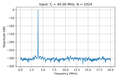
For example, using this Python script, let us set a sampling frequency, $f_{s}=40\,\mathrm {MHz}$, and generate a sinusoid with 673 periods, with the number of samples $N=2^{10}=1024$. Let us then choose a sinusoid that is an integer multiple of ${\tfrac {f_{s}}{N}}$. Thus, we get $f_{\mathrm {in} }=100\cdot {\tfrac {f_{s}}{N}}=3.90625\,\mathrm {MHz}$. The spectrum of our single sinusoid is shown in Fig. 4.

Figure 4: The spectrum of a single tone at $3.906\,\mathrm {MHz}$.

Figure 5: The spectrum of the output of a nonlinear stage.

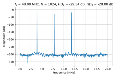
If we pass this input sinusoid through a nonlinear stage with $\alpha _{1}=10$, $\alpha _{2}=0.5$, and $\alpha _{3}=-3$, we get the spectrum in Fig. 5. As expected, we get the second and third harmonic frequency components at $7.8125\,\mathrm {MHz}$ and $11.71875\,\mathrm {MHz}$ respectively.

Note that the y-axis of Figs. 4 and 5 are normalized to the fundamental, i.e. the fundamental will always have a value of 0dB. Also, we can see that the numeric noise floor is around -300dB, due to the finite floating point range of the computer I am using. In real systems, we will be limited by electronic noise, which we will cover in the next module.

We can define the fractional harmonic distortion metric as the ratio of the amplitude of the harmonic to the fundamental. Thus, we can calculate the second fractional harmonic distortion, ($HD_{2}$), as:

$HD_{2}=20\log \left({\frac {\frac {\alpha _{2}}{2}}{\alpha _{1}+{\frac {3\alpha _{3}}{4}}}}\right)=-29.83\,\mathrm {dB}$

(4)

And the third fractional harmonic distortion, ($HD_{3}$), as:

$HD_{3}=20\log \left({\frac {\frac {\alpha _{3}}{4}}{\alpha _{1}+{\frac {3\alpha _{3}}{4}}}}\right)=-20.28\,\mathrm {dB}$

(5)

This agrees with our FFT results.

Activity 1

Modify the Python script used above to:

1. Generate the frequency spectrum of two tones with $f_{1}=100\cdot {\tfrac {f_{s}}{N}}=3.90625\,\mathrm {MHz}$ and $f_{2}=120\cdot {\tfrac {f_{s}}{N}}=4.6875\,\mathrm {MHz}$.
2. Then plot the spectrum when the two input tones are passed through a nonlinear stage with $\alpha _{1}=10$, $\alpha _{2}=0.5$, and $\alpha _{3}=-3$.
3. Compare the frequency locations of the harmonic and intermodulation tones to their theoretical locations.
4. Compare the simulated and theoretical values of the harmonic and intermodulation terms.

Submissions

Submit via email a 1-page report, excluding the graphs, detailing how you performed the steps outlined above. Include your graphs in your report.

Activity 2

Figure 6: A common-emitter amplifier.

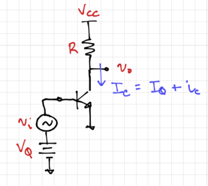
Let's look at a more practical example. Given the common-emitter amplifier shown in Fig. 6, let us calculate the collector current as a function of the input voltage. Recall that

$I_{C}=I_{S}\cdot e^{\frac {V_{BE}}{V_{T}}}$

(6)

If $V_{BE}=v_{i}+V_{Q}$, where $V_{Q}$ is the quiescent or DC voltage that results in the DC quiescent current, $I_{Q}$, express the small change in collector current, $i_{c}$ due to a small change in the base-emitter voltage, $v_{i}$, as a power series:

$i_{c}=\alpha _{0}+\alpha _{1}v_{i}+\alpha _{2}v_{i}^{2}+\alpha _{3}v_{i}^{3}+\ldots$

(7)

Hint: $e^{x}=1+x+{\tfrac {x^{2}}{2!}}+{\tfrac {x^{3}}{3!}}+\ldots$.

1. Find expressions for the values of $\alpha _{i}$ for $i=0,1,2,3$.

Submissions

Submit via email a 1-page report detailing your answer.