Information and entropy

Before We Begin ...

Some fancy art of the Brain. Made by Danknight.

From the last module's introduction, information occurs in everyday life, and it consists of two aspects: surprise and meaning. We would like to emphasize that our focus will be on the mathematics of surprise or uncertainty. Whenever you study a subject, you also experience a subtle application of information theory. For example, you are asked to review your elementary algebra again. You have confidence that the topic is easy, and you only need very little "brainpower" for the subject. It looks and feels easy because you are familiar with the material. You already have the information for the topic. Suppose you were asked to review your calculus subjects (e.g., Math 20 series) you may find it more challenging because most theories may or may not be familiar to you. There is a higher degree of uncertainty. This time you need to exert more effort in studying. If you were asked to take on a new theory that you have no clue about, you have maximum uncertainty about that theory. However, once you have given enough time and effort to study that theory, that uncertainty now becomes acquired information for you. You may not need too much brainpower to review or teach that topic again. This leads to an important concept that may repeat in future discussions. We experience an uncertainty about a topic that we don't know about. However, when we "receive" that uncertainty, it becomes information.

There is a subtle tradeoff between uncertainty and brainpower for a particular subject. You will start to notice this later in the course. Observe that when there is high uncertainty (e.g., a completely new topic), our brain exerts effort to study a material. Whenever we have low uncertainty (e.g., review a familiar subject), we exert less effort for the subject. The amount of brainpower that we use can be analogous to computing power. The uncertainty can be associated with the data that we need to process. This example shows where information theory and complexity mix together. If we are given a similar problem, what would the best solution be? Information theory does not tell us how to solve a problem because it is only a measurement. The solutions are up to us. Going back to our study example, if we need to study a completely new topic, what are our options? Do we spend so much time on the material to cover the bulk of it? How much brainpower do we use? Or can we cut the material into chunks so that we can process it with optimum time and power? The solution is up to us. We just need to be creative.

Chunking is a well-known learning strategy to reduce the workload on a particular subject. It is proven to be effective in studying new topics. You can find several Youtube videos on chunking. Go ahead and try.

Deriving Information

Shannon has a very nice comprehensive introduction on how he formulated his theory . Let's try to summarize his approach in a different way . Remember, our mathematical definition of information is the measurement of surprise. Let's say we have an experiment with two independent events $e$ and $f$. Shannon pointed out important properties of information:

1. $I(e)$ should be a decreasing function of $P(e)$. The same goes for event $f$.
2. If the two events have $P(e)\leq P(f)$ then it should follow that $I(e)\geq I(f)$. Again, following that the more surprising event should have higher information.
3. Since both events are independent, then $I(e\cap f)=I(e)+I(f)$. Also, following from the previous item: $I(e\cap f)\geq I(e)\geq I(f)$.

Let's look at a simple example. Suppose we'll be drawing a card from a pack of 52 casino cards. Suppose we have we get the probabilities where the drawn card is:

• A club. Let this be event $a$.
• An ace. Let this be event $b$.
• An ace of clubs. Let this be event $a\cap b$.

The equivalent probabilities would be:

• $P(a)={\frac {1}{4}}$
• $P(b)={\frac {1}{13}}$
• $P(a\cap b)={\frac {1}{52}}$

Since we know the probabilities and the desired properties for Shannon's theorem, we can observe the following. $I(a)\geq I(b)$ because it is more surprising to draw an ace compared to drawing any card that is a club. $I(a\cap b)\geq I(a)\geq I(b)$ because it is a lot more surprising to get the ace of clubs compared to the individual events. Moreover, our intuition tells us that $I(a\cap b)=I(b)+I(a)$. The question is, what kind of function should information be if we know the probabilities of each event? After hours of thinking, Shannon came up with:

$I(x)=\log _{2}\left({\frac {1}{P(x)}}\right)$

(1)

Which can also be re-written as the equation below because of the law of logarithms $\log _{a}(x^{n})=n\log _{a}(x)$.

$I(x)=-\log _{2}\left(P(x)\right)$

(1)

So either way works and we'll call them equation 1. Let's apply these in action, if we calculate the information for events $a$, $b$, and $a\cap b$.

• $I(a)=-{\frac {1}{4}}\log _{2}\left({\frac {1}{4}}\right)=2\ {\textrm {bits}}$
• $I(b)=-{\frac {1}{13}}\log _{2}\left({\frac {1}{13}}\right)=3.70\ {\textrm {bits}}$
• $I(a\cap b)=-{\frac {1}{52}}\log _{2}\left({\frac {1}{52}}\right)=5.70\ {\textrm {bits}}$

It satisfies everything we agreed upon!

• $I(b)\geq I(a)\rightarrow 3.70\geq 2.00$
• $I(a\cap b)\geq I(b)\geq I(a)\rightarrow 5.70\geq 3.70\geq 2.00$
• $I(a\cap b)=I(b)+I(a)=3.70+2.00=5.70$

It's simple and it agrees well. There's a special case say $P(x)=0$ for some event $x$. This leads to $\log _{2}(0)\rightarrow \infty$. This breaks those assumptions that Shannon made. Because of this we'll have to make an exemption where $P(x)=0$ then $I(x)=0$. So equation 1 is more appropriately written as:

$I(x)={\begin{cases}-\log _{2}\left(P(x)\right)&P(x)>0\\0&P(x)=0\end{cases}}$

(1)

Bits, Bans, and Nats

You might wonder why we used base 2 for the log function. This is just for convenience because using the equation in base 2 suits well with our binary computations. The units of information if taken in base 2 are in bits. If taken in base 3 we call them trits. If taken in base 10 we call them bans, and if taken in base $e$, we call them nats. The table below shows this comparison.

base	units	$I(0.25)$
2	bits (from binary)	2.00
3	trits (from trinary)	1.26
$e$	nats (from natural logarithm)	1.38
10	bans	0.602

Information Examples

In summary, information can be thought of as the amount of surprise at seeing an event. Note that a highly probable outcome is not surprising. Consider the following events:

Event	Probability	Information (Surprise)
Someone tells you $1=1$.	$1$	$\log _{2}\left(1\right)=0$
You got the wrong answer on a 4-choice multiple choice question.	${\frac {3}{4}}$	$\log _{2}\left({\frac {4}{3}}\right)=0.415\,\mathrm {bits}$
You guessed correctly on a 4-choice multiple choice question.	${\frac {1}{4}}$	$\log _{2}\left(4\right)=2\,\mathrm {bits}$
You got the correct answer in a True or False question.	${\frac {1}{2}}$	$\log _{2}\left(2\right)=1\,\mathrm {bit}$
You rolled a seven on rolling a pair of dice.	${\frac {6}{36}}$	$\log _{2}\left(6\right)=2.58\,\mathrm {bits}$
Winning the Ultra Lotto 6/58 jackpot.	${\frac {1}{40400000}}$	$\log _{2}\left(40400000\right)=25.27\,\mathrm {bits}$

Try it yourself. Find something where you can measure information. Ponder on the question "How surprising is this event?".

Entropy

Information is a measure of surprise for one event only. We are also interested in a collection of events encapsulated with some random variable $X$. Recall that a random variable contains a set of outcomes $\{x_{1},x_{2},x_{3},...,x_{n}\}$ and each outcome has an associated probability $\{P(x_{1}),P(x_{2}),P(x_{3}),...,P(x_{n})\}$. Each outcome also has its own set of information $\{I(x_{1}),I(x_{2}),I(x_{3}),...,I(x_{n})\}$. We can get the mean of all $I(X)$. We call this entropy which we denote with $H(X)$:

$H(X)=E(I(X))=-\sum _{i=1}^{n}P(x_{i})\log _{2}\left(P(x_{i})\right)$

(2)

Entropy is literally just the mean of information for some random variable $X$. Let's look at a few examples. Consider some random variable $X$ with outcomes $\{x_{1},x_{2},x_{3},x_{4},x_{5},x_{6},x_{7},x_{8}$. All outcomes have a probability of $\{P(x_{1})=P(x_{2})=P(x_{3})=P(x_{4})=P(x_{5})=P(x_{6})=P(x_{7})=P(x_{8})={\frac {1}{8}}\}$. What is $H(X)$? Simple!

${\begin{aligned}H(X)&=-\sum _{i=1}^{n}P(x_{i})\log _{2}\left(P(x_{i})\right)\\&=-8\cdot {\frac {1}{8}}\log _{2}\left({\frac {1}{8}}\right)\\&=3.00\ {\textrm {bits}}\end{aligned}}$

Therefore, the average information for the simple uniform distribution is $3.00$ bits. Let's take a look at another example. Suppose we flip a fair coin three times. Let the random variable $X$ be the sum of heads in those three flips. What is $H(X)$? It's easier to tabulate the data.

$x_{i}$	$P(X=x_{i})$	$I(X=x_{i})$	$P(X=x_{i})I(X=x_{i})$
$0$	${\frac {1}{8}}$	$3.00$	$0.375$
$1$	${\frac {3}{8}}$	$1.415$	$0.531$
$2$	${\frac {3}{8}}$	$1.415$	$0.531$
$3$	${\frac {1}{8}}$	$3.00$	$0.375$

Summing all $P(X=x_{i})I(X=x_{i})$ terms we get:

$H(X)=P(X=0)I(X=0)+P(X=1)I(X=1)+P(X=2)I(X=2)+P(X=3)I(X=3)=1.81\ {\textrm {bits}}$

Bounds of Entropy

Entropy has bounds, meaning there is a lower and upper limit to this value. Just like in any system, these bounds serve as limitations to our measurement. In a nutshell, for any random variable $X$ with $n$ outcomes, the bounds of entropy is:

$0\geq H(X)\geq \log(n)$

(3)

The lower bound $H(X)\geq 0$ occurs if and only if one of the outcomes has absolute certainty (i.e., $P(X=x_{i})=1$). This is trivial. Recall that for a random variable $X$ with outcomes $\{x_{1},x_{2},...,x_{n}\}$ and their associated probabilities $\{P(x_{1}),P(x_{2}),...,P(x_{n})\}$. The sum of all probabilities must sum up to 1. Such that:

$\sum _{i=1}^{n}P(X=x_{i})=1$

Figure 1: The plot of $y=\ln \left(x\right)$ and $y=x-1$.

If one of the elements has absolute certainty: $P(X=x_{i})=1$ then that means all other probabilities need to be $P(X=x_{j})=0$ where $i\neq j$. Solving for $H(X)=0$ if this happens.

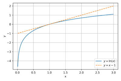
The upper bound is a bit tricky. First we need to recognize a fact that $\ln(x)\leq x-1$ with equality if and only if $x=1$. When we say "with equality" then that means the equal sign holds true if and only if the condition is met. This is trivial: $\ln(x)\leq x-1\rightarrow \ln(1)=1-1\rightarrow 0=0$ if and only if $x=1$. We can also observe $\ln(x)$ and $x-1$ from figure 1.

Second, we need to appreciate what Gibbs inequality tells us. Suppose we have two probability distributions $P=\{p_{1},p_{2},...,p_{n}\}$ and $Q=\{q_{1},q_{2},...,q_{n}\}$. Also note that $\sum _{i=1}^{n}p_{i}=1$ and $\sum _{i=1}^{n}q_{i}=1$. Gibbs inequality says:

$\sum _{i=1}^{n}p_{i}\ln \left({\frac {q_{i}}{p_{i}}}\right)\leq \sum _{i=1}^{n}p_{i}\left({\frac {q_{i}}{p_{i}}}-1\right)$

(4)

Simplifying the right handside results in:

$\sum _{i=1}^{n}\left(q_{i}-p_{i}\right)=\sum _{i=1}^{n}q_{i}-\sum _{i=1}^{n}p_{i}=1-1=0$

In other words, Gibbs inequality says that:

$\sum _{i=1}^{n}p_{i}\ln \left({\frac {q_{i}}{p_{i}}}\right)=0$

(5)

If and only if $p_{i}=q_{i}$ for all $i$. Take note of equation 5 and its condition for being true. We will use this result for deriving the upper bound. Now, let's consider a random variable $X$ with probability distribution $P=\{p_{1},p_{2},...,p_{n}\}$. Let's find what kind of distribution maximizes the entropy function. We have:

${\begin{aligned}H(P)-\log(n)&=\sum _{i=1}^{n}p_{i}\log \left({\frac {1}{p_{i}}}\right)-\log(n)\\&=\sum _{i=1}^{n}p_{i}\log \left({\frac {1}{p_{i}}}\right)-\sum _{i=1}^{n}p_{i}\log(n)\\&=\sum _{i=1}^{n}p_{i}\left(\log \left({\frac {1}{p_{i}}}\right)-\log(n)\right)\\&=\sum _{i=1}^{n}p_{i}\log \left({\frac {\frac {1}{n}}{p_{i}}}\right)\\&\leq 0\end{aligned}}$

The second step works because we know that $\sum _{i=1}^{n}p_{i}=1$. The last step works because of Gibbs inequality (i.e., $\sum _{i=1}^{n}p_{i}\ln \left({\frac {q_{i}}{p_{i}}}\right)=0$). Therefore $H(P)-\log(n)=0$ works if and only if $p_{i}={\frac {1}{n}}$ for all $i$.

In plain English, this means that we attain maximum entropy if and only if all outcomes are equiprobable!

In summary, the bounds of entropy can be summarized as $0\geq H(X)\geq \log(n)$.

• The lower bound occurs if at least one outcome has absolute certainty $p_{i}=1$.
• The upper bound occurs if all outcomes are equiprobable $p_{i}={\frac {1}{n}}$. Assuming there are $n$ outcomes.

References

- ↑ Sousa, David A. 2006. How the Brain Learns. Thousand Oaks, Calif: Corwin Press.
- ↑ Shannon, C. E., & Weaver, W., The mathematical theory of communication. Urbana: University of Illinois Press. 1949.
- ↑ Applebaum, D. , Probability and Information: An Integrated Approach, Cambridge University Press, 2008.